The HPSPLIT Procedure

PROC HPSPLIT Statement
-
PROC HPSPLIT <options>;
The PROC HPSPLIT statement invokes the procedure. Table 61.1 summarizes the options in the PROC HPSPLIT statement.
Table 61.1: PROC HPSPLIT Statement Options
|
Option |
Description |
|---|---|
|
Basic Options |
|
|
Requests a table of the results of cost-complexity pruning based on cross validation |
|
|
Specifies the cross validation method to use |
|
|
Requests model assessment and a confusion matrix with cross validation |
|
|
Specifies the predictor data set |
|
|
Specifies the number of bins for continuous variables |
|
|
Sets the minimum variance for a regression tree leaf to be split |
|
|
Requests a table that describes the nodes of the final tree |
|
|
Suppresses ODS output |
|
|
Specifies the number of surrogate rules to create |
|
|
Specifies options for plots |
|
|
Specifies the random number seed to use for cross validation |
|
|
Specifies that variables should be split only once per branch |
|
|
Splitting Options |
|
|
Specifies how to handle missing values in a predictor variable |
|
|
Specifies the maximum number of computations to perform in an exhaustive search for a categorical predictor |
|
|
Specifies the number of computations to perform before the splitter uses the fastest greedy search |
|
|
Specifies the maximum number of leaves per node |
|
|
Specifies the maximum tree depth |
|
|
Specifies the number of observations per level in order for the level to be considered for splitting |
|
|
Specifies the minimum number of observations per leaf |
|
You can specify the following options.
- ASSIGNMISSING=BRANCH NONE POPULAR SIMILAR
-
specifies how PROC HPSPLIT creates a default splitting rule to handle missing values, unknown levels, and levels that have fewer observations than you specify in the MINCATSIZE= option. An unknown level is a level of a categorical predictor that does not exist in the training data but is encountered during scoring.
Both the ASSIGNMISSING= and NSURROGATES= options affect training and scoring. See the NSURROGATES= option for the definition of surrogate rules.
During training, the primary splitting rule is created first, along with the default splitting rule (controlled by the ASSIGNMISSING= option). If you request surrogate rules (by using the NSURROGATES= option), they are created after the primary and default splits are made. When the splitting rules have been created, the rules are used as described in the following list for assigning the training data by using the new splitting rules, and splitting rule creation continues on the new children.
Observation assignment during the training phase and during scoring proceeds as follows:
-
The primary splitting rule is applied if the rule’s variable is not missing. Otherwise:
-
The first surrogate rule (with the largest agreement, described in the section Primary and Surrogate Splitting Rules) is applied if the first surrogate rule’s variable is not missing. Otherwise:
-
Each subsequent (ordered by agreement) splitting rule is applied as described in the first surrogate item in this list. If all of the surrogate rules’ variables are missing, then:
-
The default splitting rule is used.
Because there is always a default splitting rule, all data can be scored, even if the primary rule and all surrogate rules cannot be used on a particular observation.
You can specify one of the following:
By default, ASSIGNMISSING=NONE.
-
-
CVCC
CVCOSTCOMPLEXITY -
requests a table of the results of cost-complexity pruning based on cross validation. For each fold in the cross validation, the table provides the penalty parameter, the number of leaves, and the average ASE. In addition, the table provides the minimum and maximum ASE, and the minimum, median, and maximum number of leaves. The number of leaves is the floor of the median. You can use the PLOTS=CVCC option to request a plot of the information in this table.
- CVMETHOD=NONE RANDOM <(k)>
-
requests the cross validation method to be performed.
You can specify one of the following:
By default, CVMETHOD=RANDOM(10) when you perform cost-complexity pruning with no PARTITION statement.
- CVMODELFIT
-
requests model assessment with cross validation. When you specify this option, the procedure does a cross validation of the final model parameters and produces a table that describes the cross validation error measures of the parameters. The table contains various summary statistics of the ASE, the number of leaves, and, for a categorical response, the misclassification rate across the k trees grown. This option also requests a table that contains the cross validation confusion matrix.
If cost complexity is cross validated (the default if you use cost-complexity pruning without a validation set), the assessment is a completely separate cross validation of the final tree penalty parameter, using a different seed for fold assignment.
Note: The assessment is not on a holdout sample but instead on k-fold cross validation. This is not a second run of the procedure but instead is done automatically and internally.
- DATA=SAS-data-set
-
names the predictor SAS data set to be used by PROC HPSPLIT. The default is the most recently created data set.
If the procedure executes in distributed mode, the predictor data are distributed to memory on the appliance nodes and analyzed in parallel, unless the data are already distributed in the appliance database. In that case, the procedure reads the data alongside the distributed database. For more information, see the section Processing Modes in SAS/STAT 14.1 User's Guide: High-Performance Procedures about the various execution modes and the section Alongside-the-Database Execution in SAS/STAT 14.1 User's Guide: High-Performance Procedures about the alongside-the-database model.
- INTERVALBINS=number
-
specifies the number of bins for continuous variables. PROC HPSPLIT bins continuous predictors to a fixed bin size. This option controls the number of bins and thereby also the size of the bins. For more information about interval variable binning, see the section Details: HPSPLIT Procedure.
By default, INTERVALBINS=100.
- LEVTHRESH1=number
-
applies only to categorical predictor variables and specifies the limit for the number of computations in an exhaustive search for the optimal partition of the levels of a particular variable. The splitter first evaluates the number of computations that are needed for an exhaustive search. If this number exceeds the limit, then the splitter falls back to a faster heuristic algorithm. You can use the LEVTHRESH2= option to specify the limit for the number of computations in this faster algorithm.
By default, LEVTHRESH1=500000.
- LEVTHRESH2=number
-
applies to categorical predictor variables and continuous predictor variables with multiway splits. This option does not apply to continuous predictor variables with binary splits.
For a categorical predictor variable, the splitter first evaluates the number of computations that are needed for an exhaustive search. If this number exceeds the limit that you specify in the LEVTHRESH1= option, then the splitter falls back to a faster heuristic algorithm. You can use the LEVTHRESH2= option to specify the limit for the number of computations in this faster algorithm. If this number of computations exceeds the limit that you specify in the LEVTHRESH2= option, then the splitter falls back to an even faster algorithm.
For a continuous predictor variable, the splitter first tries to perform an exhaustive search for the optimal split values. The splitter first evaluates the number of computations that are needed for an exhaustive search. If this number exceeds the limit that you specify in the LEVTHRESH2= option, the splitter falls back to a faster heuristic algorithm.
By default, LEVTHRESH2=1000000.
- MAXBRANCH=b
-
specifies the maximum number of children per node in the tree. PROC HPSPLIT tries to create this number of children unless it is impossible (for example, if a split variable does not have enough levels). By default, MAXBRANCH=2.
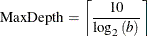
- MAXDEPTH=number
-
specifies the maximum depth of the tree to be grown. The default is set using the following equation, where b is the value for the MAXBRANCH= option:
- MINCATSIZE=number
-
specifies the number of observations that a categorical variable level must have in order to be considered in the split. Predictor variable levels that have fewer observations than number receive the nonsurrogate missing value assignment for that split. See the NSURROGATES= option for the definition of surrogate rules.
By default, MINCATSIZE=1.
- MINLEAFSIZE=number
-
specifies the minimum number of observations that each child of a split must contain in the training data set in order for the split to be considered.
By default, MINLEAFSIZE=1.
- MINVARIANCE=value
-
specifies the minimum variance for a regression tree leaf to be eligible for splitting. That is, leaves whose variance is less than value are not split any further.
By default, MINVARIANCE=1E–8.
The variance at some leaf
 with weight
  (number of observations) is calculated using
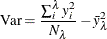
where
 is the response value at observation i and
  is the average value of the response within leaf .
- NODES=DETAIL SUMMARY
-
requests a table that contains the description of the paths from each leaf to the root.
You can specify the following values:
- NOPRINT
- NSURROGATES=number
-
specifies the number of surrogate rules to create for each splitting rule. Surrogate rules are backup splitting rules that are used when the variable that corresponds to the primary splitting rule is missing. By default, NSURROGATES=0.
Both the ASSIGNMISSING= option and NSURROGATES= options affect training and scoring.
During training, the primary splitting rule is created first, along with the default splitting rule (controlled by the ASSIGNMISSING= option). If you request surrogate rules (by specifying the NSURROGATES= option), they are created after the primary and default splits are created. When the splitting rules have been created, the rules are used as described in the following list for assigning the training data by using the new splitting rules, and splitting rule creation continues on the new children.
Observation assignment during the training phase and during scoring proceeds as follows:
-
The primary splitting rule is applied if the primary rule’s variable is not missing. Otherwise:
-
The first surrogate rule (with the largest agreement, described in the section Primary and Surrogate Splitting Rules) is applied if the first surrogate rule’s variable is not missing. Otherwise:
-
Each subsequent (ordered by agreement) splitting rule is applied as described in the first surrogate item in the list. If all of the surrogate rules’ variables are missing, then:
-
The default splitting rule is used.
Because there is always a default splitting rule, all data can be scored, even if the primary rule and all surrogate rules cannot be used on a particular observation.
As auxiliary rules, surrogate rules are used in the following ways:
-
Surrogate rules are used in generating the tree.
-
Surrogate rules therefore also affect the final tree metrics.
-
Surrogate rules are used in the SAS code output from the CODE statement.
-
Surrogate rules are used in scoring the predictor data set by using the OUTPUT statement.
-
Surrogate rules are not written out in the “Node Rules” file, output from the RULES statement.
-
-
PLOTS <(global-plot-option)> <= plot-request <(options)>>
PLOTS <(global-plot-option)> <= (plot-request <(options)> <... plot-request <(options)>>)> -
controls the plots that are produced through ODS Graphics. When you specify only one plot-request, you can omit the parentheses around it. Some examples follow.
You can specify the following global-plot-option:
You can specify the following plot-requests:
- SEED=number
-
specifies the initial seed for random number generation for cross validation. The value of number must be an integer. The default seed is based on the date and time.
- SPLITONCE
-
specifies that variables be split only once on a branch. However, a variable can be used more than once across branches. That is, a variable cannot be split more than once on the path from any leaf to the root node.