The HPSPLIT Procedure

Getting Started: HPSPLIT Procedure
This example explains basic features of the HPSPLIT procedure for building a classification tree. The data are measurements of 13 chemical attributes for 178 samples of wine. Each wine is derived from one of three cultivars that are grown in the same area of Italy, and the goal of the analysis is a model that classifies samples into cultivar groups. The data are available from the UCI Irvine Machine Learning Repository; see Bache and Lichman (2013).
The following statements create a data set named Wine that contains the measurements:
data Wine;
   %let url = http://archive.ics.uci.edu/ml/machine-learning-databases;
   infile "&url/wine/wine.data" url delimiter=',';
   input Cultivar Alcohol Malic Ash Alkan Mg TotPhen
         Flav NFPhen Cyanins Color Hue ODRatio Proline;
   label Cultivar = "Cultivar"
         Alcohol  = "Alcohol"
         Malic    = "Malic Acid"
         Ash      = "Ash"
         Alkan    = "Alkalinity of Ash"
         Mg       = "Magnesium"
         TotPhen  = "Total Phenols"
         Flav     = "Flavonoids"
         NFPhen   = "Nonflavonoid Phenols"
         Cyanins  = "Proanthocyanins"
         Color    = "Color Intensity"
         Hue      = "Hue"
         ODRatio  = "OD280/OD315 of Diluted Wines"
         Proline  = "Proline";
run;

proc print data=Wine(obs=10); run;
Figure 61.1 lists the first 10 observations of Wine.
Figure 61.1: Partial Listing of Wine
| Obs | Cultivar | Alcohol | Malic | Ash | Alkan | Mg | TotPhen | Flav | NFPhen | Cyanins | Color | Hue | ODRatio | Proline |
|---|---|---|---|---|---|---|---|---|---|---|---|---|---|---|
| 1 | 1 | 14.23 | 1.71 | 2.43 | 15.6 | 127 | 2.80 | 3.06 | 0.28 | 2.29 | 5.64 | 1.04 | 3.92 | 1065 |
| 2 | 1 | 13.20 | 1.78 | 2.14 | 11.2 | 100 | 2.65 | 2.76 | 0.26 | 1.28 | 4.38 | 1.05 | 3.40 | 1050 |
| 3 | 1 | 13.16 | 2.36 | 2.67 | 18.6 | 101 | 2.80 | 3.24 | 0.30 | 2.81 | 5.68 | 1.03 | 3.17 | 1185 |
| 4 | 1 | 14.37 | 1.95 | 2.50 | 16.8 | 113 | 3.85 | 3.49 | 0.24 | 2.18 | 7.80 | 0.86 | 3.45 | 1480 |
| 5 | 1 | 13.24 | 2.59 | 2.87 | 21.0 | 118 | 2.80 | 2.69 | 0.39 | 1.82 | 4.32 | 1.04 | 2.93 | 735 |
| 6 | 1 | 14.20 | 1.76 | 2.45 | 15.2 | 112 | 3.27 | 3.39 | 0.34 | 1.97 | 6.75 | 1.05 | 2.85 | 1450 |
| 7 | 1 | 14.39 | 1.87 | 2.45 | 14.6 | 96 | 2.50 | 2.52 | 0.30 | 1.98 | 5.25 | 1.02 | 3.58 | 1290 |
| 8 | 1 | 14.06 | 2.15 | 2.61 | 17.6 | 121 | 2.60 | 2.51 | 0.31 | 1.25 | 5.05 | 1.06 | 3.58 | 1295 |
| 9 | 1 | 14.83 | 1.64 | 2.17 | 14.0 | 97 | 2.80 | 2.98 | 0.29 | 1.98 | 5.20 | 1.08 | 2.85 | 1045 |
| 10 | 1 | 13.86 | 1.35 | 2.27 | 16.0 | 98 | 2.98 | 3.15 | 0.22 | 1.85 | 7.22 | 1.01 | 3.55 | 1045 |
The variable Cultivar is a nominal categorical variable with levels 1, 2, and 3, and the 13 attribute variables are continuous.
The following statements use the HPSPLIT procedure to create a classification tree:
ods graphics on;

proc hpsplit data=Wine seed=15531;
   class Cultivar;
   model Cultivar = Alcohol Malic Ash Alkan Mg TotPhen Flav
                    NFPhen Cyanins Color Hue ODRatio Proline;
   grow entropy;
   prune costcomplexity;
run;
The MODEL statement specifies Cultivar as the response variable and the variables to the right of the equal sign as the predictor variables. The inclusion of Cultivar in the CLASS statement designates it as a categorical response variable and requests a classification tree. All the predictor
variables are treated as continuous variables because none are included in the CLASS statement.
The GROW and PRUNE statements control two fundamental aspects of building classification and regression trees: growing and pruning. You use the GROW statement to specify the criterion for recursively splitting parent nodes into child nodes as the tree is grown. For classification trees, the default criterion is entropy; see the section Splitting Criteria.
By default, the growth process continues until the tree reaches a maximum depth of 10 (you can specify a different limit by using the MAXDEPTH= option). The result is often a large tree that overfits the data and is likely to perform poorly in predicting future data. A recommended strategy for avoiding this problem is to prune the tree to a smaller subtree that minimizes prediction error. You use the PRUNE statement to specify the method of pruning. The default method is cost complexity; see the section Pruning.
The default output includes the four informational tables that are shown in Figures Figure 61.2 through Figure 61.5.
The "Performance Information" table in Figure 61.2 shows that the procedure executes in single-machine mode—that is, all the computations are done on the machine where the SAS session executes. This run of the HPSPLIT procedure was performed on a multicore machine with the same number of CPUs as there are threads; that is, one computational thread was spawned per CPU.
Figure 61.2: Performance Information
The "Data Access Information" table in Figure 61.3 shows that the input data set is accessed using the V9 (base) engine on the client machine where the MVA SAS session executes. This table includes similar information about output data sets that you can request by using the OUTPUT statement.
Figure 61.3: Data Access Information
The "Model Information" table in Figure 61.4 provides information about the model and the methods that are used to grow and prune the tree.
Figure 61.4: Model Information
The "Observation Information" table in Figure 61.5 provides the numbers of observations that are read and used.
Figure 61.5: Observation Information
These numbers are the same in this example because there are no missing values in the predictor variables. By default, observations that have missing values are not used. However, the HPSPLIT procedure provides methods for incorporating missing values in the analysis, as explained in the sections Handling Missing Values and Primary and Surrogate Splitting Rules.
The plot in Figure 61.6 is a tool for selecting the tuning parameter for cost-complexity pruning. The parameter, indicated on the lower horizontal axis, indexes a sequence of progressively smaller subtrees that are nested within the large tree. The parameter value 0 corresponds to the large tree, and positive values control the trade-off between complexity (number of leaves) and fit to the training data, as measured by average square error (ASE).
Figure 61.6: Cost-Complexity Plot
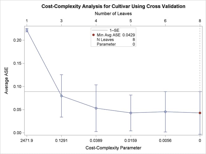
Figure 61.6 shows that PROC HSPLIT selects the parameter value 0 because it minimizes the estimate of ASE, which is obtained by 10-fold cross validation. However, the ASEs for several other parameter choices are nearly the same.
Breiman’s 1-SE rule chooses the parameter that corresponds to the smallest subtree for which the predicted error is less than one standard error above the minimum estimated ASE (Breiman et al. 1984). This parameter choice (0.1291) corresponds to a very small tree that has only three leaves.
Note: The estimates of ASE and their standard errors depend on the random assignment of observations to the folds in the cross validation, which is determined by the SEED= option.
The following statements build a classification tree by growing a large tree and applying cost-complexity pruning (also known as weakest-link pruning) to obtain a tree that has three leaves:
proc hpsplit data=Wine seed=15531;
   class Cultivar;
   model Cultivar = Alcohol Malic Ash Alkan Mg TotPhen Flav
                    NFPhen Cyanins Color Hue ODRatio Proline;
   prune costcomplexity(leaves=3);
run;
The tree diagram in Figure 61.7, which is produced by default when ODS Graphics is enabled, provides an overview of the tree as a classifier.
Figure 61.7: Overview Diagram of Final Tree
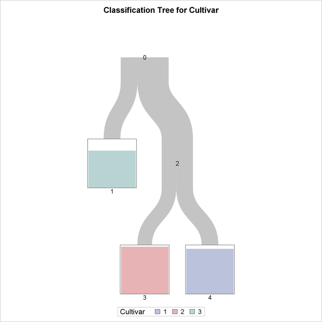
The tree is constructed starting with all the observations in the root node (labeled 0). This node is split into a leaf node (1) and an internal node (2), which is further split into two leaf nodes (3 and 4).
The color of the bar in each leaf node indicates the most frequent level of Cultivar among the observations in that node; this is also the classification level assigned to all observations in that node. The
height of the bar indicates the proportion of observations in the node that have the most frequent level. The width of the
link between parent and child nodes is proportional to the number of observations in the child node.
The diagram reveals that splitting on just two of the attributes is sufficient to differentiate the three cultivars, and a tree model that has only three leaves provides a high degree of accuracy for classification.
The diagram in Figure 61.8 provides more detail about the nodes and the splits.
Figure 61.8: Detailed Tree Diagram
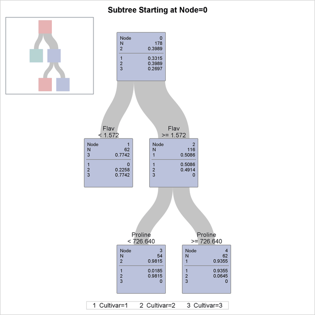
There are 178 samples in the root node (node 0). The table below the line in the box for node 0 provides the proportion of
samples for each level of Cultivar, and the level that has the highest proportion is also given above the line. These samples are divided into 62 samples for
which Flav  (node 1) and 116 samples for which
 Flav  (node 2).
The variable Flav and the split point 1.572 are chosen to maximally decrease the impurity of the root node as measured by the entropy criterion.
There are no samples for which Cultivar=1 in node 1, and there are no samples for which Cultivar=3 in node 2.
The samples in node 2 were further divided into 54 samples for which Proline < 726.640 (node 3) and 62 samples for which Proline  (node 4).
The classification tree yields simple rules for predicting the wine cultivar. For example, a sample for which Flav and Proline < 726.640 is predicted to be from the third cultivar (Cultivar=3).
The diagram in Figure 61.8 happens to show the entire tree that was created by the preceding statements, but in general this diagram shows a subtree of the entire tree that begins with the root node and has a depth of four levels. You can use the PLOTS=ZOOMEDTREE option in the PROC HPSPLIT statement to request diagrams that begin with other nodes and have specified depths.
The confusion matrix in Figure 61.9 evaluates the accuracy of the fitted tree for classifying the training data that were used to build the tree model.
Figure 61.9: Confusion Matrix
The values in the off-diagonal entries of the matrices show how many times the fitted model misclassified a sample. For example,
among the 59 samples for which Cultivar=1, only one sample was misclassified, and it was incorrectly classified as Cultivar=2.
The "Tree Performance" table in Figure 61.10 displays various fit statistics for the tree model.
Figure 61.10: Fit Statistics
For instance, the misclassification rate is the proportion of the 178 wine samples that were misclassified: (1 + 4 + 14)/178 = 0.1067.
You can use the CVMODELFIT option in the PROC HPSPLIT statement to request a model assessment that is based on cross validation; this is done independently of the cross validation used to assess pruning parameters. For more information about fit statistics, see the section Measures of Model Fit.
Note: Additional fit statistics are available in the case of classification trees for binary responses. See Building a Classification Tree for a Binary Outcome.