The HPSPLIT Procedure

This example performs an analysis similar to the one in the "Getting Started" section of Chapter 60: The HPREG Procedure, where a linear regression model is fit. You can alternatively fit a regression tree to predict the salaries of Major League Baseball players based on their performance measures from the previous season by using almost identical code. Regression trees are piecewise constant models that, for relatively small data sets such as this, provide succinct summaries of how the predictors determine the predictions. These models are usually easier to interpret than linear regression models. The Sashelp.Baseball data set contains salary and performance information for Major League Baseball players (excluding pitchers) who played at least one game in both the 1986 and 1987 seasons (Time Inc. 1987). The following statements create a regression tree model:

ods graphics on;

proc hpsplit data=sashelp.baseball seed=123;
   class league division;
   model logSalary = nAtBat nHits nHome nRuns nRBI nBB
                     yrMajor crAtBat crHits crHome crRuns crRbi
                     crBB league division nOuts nAssts nError;
   output out=hpsplout;
run;

By default, the tree is grown using the RSS criterion, and cost-complexity pruning with 10-fold cross validation is performed. The OUTPUT statement requests generation of the data set hpsplout, which contains the predicted salary from the tree model for each observation.

Much of the output for a regression tree is identical to the output for a classification tree. Tables and plots where there are differences are displayed and discussed on the following pages.

Output 61.3.1 displays the full regression tree.

Output 61.3.1: Overview Diagram of Regression Tree

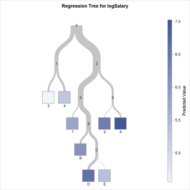
You can see from this diagram that the final selected tree has eight leaves. For a regression tree, the shade of the leaves represents the predicted response value, which is the average observed logSalary for the observations in that leaf. Node 3 has the lowest predicted response value, indicated by the lightest shade of blue, and Node A has the highest, indicated by the dark shade.

Output 61.3.2 shows details of the tree.

Output 61.3.2: Detailed Diagram of Regression Tree

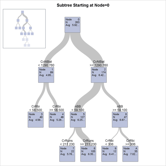
As with a classification tree, you can see split variables and values for a portion of the tree in this view. You can also see the exact predicted response value, which is the average observed response, in each node.

The confusion matrix is omitted from the output when you are modeling a regression tree because it is relevant only for a categorical response.

Output 61.3.3 displays fit statistics for the final regression tree.

Note that this table contains different statistics from those included for a classification tree. The ASE and RSS are reported here to help you assess the model fit. You could also use the CVMODELFIT option in the PROC HPSPLIT statement to obtain the cross validated fit statistics, as with a classification tree.

Output 61.3.4 shows the hpsplout data set that is created by using the OUTPUT statement and contains the first 10 observations of the predicted log-transformed salaries for each player in Sashelp.Baseball based on the regression tree model.

The variable P_logSalary contains the predicted salaries on the log scale. Note that all observations in the same leaf have the same predicted response. The OUT= data set can contain additional variables from the DATA= data set if you specify them in the ID statement.