The GENMOD Procedure

Example 44.8 Model Assessment of Multiple Regression Using Aggregates of Residuals

This example illustrates the use of cumulative residuals to assess the adequacy of a normal linear regression model. Neter et al. (1996, Section 8.2) describe a study of 54 patients undergoing a certain kind of liver operation in a surgical unit. The data consist of the survival time and certain covariates. After a model selection procedure, they arrived at the following model:

$Y = \beta _0 + \beta _1 X_1 + \beta _2 X_2 + \beta _3 X_3 + \epsilon$

where Y is the logarithm (base 10) of the survival time; $X_1$ , $X_2$ , $X_3$ are blood-clotting score, prognostic index, and enzyme function, respectively; and $\epsilon$ is a normal error term. A listing of the SAS data set containing the data is shown in Output 44.8.1. The variables Y, X1, X2, and X3 correspond to Y, $X_1$ , $X_2$ , and $X_3$ , and LogX1 is log( $X_1$ ). The PROC GENMOD fit of the model is shown in Output 44.8.2. The analysis first focuses on the adequacy of the functional form of $X_1$ , blood-clotting score.

Output 44.8.1: Surgical Unit Example Data

Obs	Y	X1	X2	X3	LogX1
1	2.3010	6.7	62	81	0.82607
2	2.0043	5.1	59	66	0.70757
3	2.3096	7.4	57	83	0.86923
4	2.0043	6.5	73	41	0.81291
5	2.7067	7.8	65	115	0.89209
6	1.9031	5.8	38	72	0.76343
7	1.9031	5.7	46	63	0.75587
8	2.1038	3.7	68	81	0.56820
9	2.3054	6.0	67	93	0.77815
10	2.3075	3.7	76	94	0.56820
11	2.5172	6.3	84	83	0.79934
12	1.8129	6.7	51	43	0.82607
13	2.9191	5.8	96	114	0.76343
14	2.5185	5.8	83	88	0.76343
15	2.2253	7.7	62	67	0.88649
16	2.3365	7.4	74	68	0.86923
17	1.9395	6.0	85	28	0.77815
18	1.5315	3.7	51	41	0.56820
19	2.3324	7.3	68	74	0.86332
20	2.2355	5.6	57	87	0.74819
21	2.0374	5.2	52	76	0.71600
22	2.1335	3.4	83	53	0.53148
23	1.8451	6.7	26	68	0.82607
24	2.3424	5.8	67	86	0.76343
25	2.4409	6.3	59	100	0.79934
26	2.1584	5.8	61	73	0.76343
27	2.2577	5.2	52	86	0.71600
28	2.7589	11.2	76	90	1.04922
29	1.8573	5.2	54	56	0.71600
30	2.2504	5.8	76	59	0.76343
31	1.8513	3.2	64	65	0.50515
32	1.7634	8.7	45	23	0.93952
33	2.0645	5.0	59	73	0.69897
34	2.4698	5.8	72	93	0.76343
35	2.0607	5.4	58	70	0.73239
36	2.2648	5.3	51	99	0.72428
37	2.0719	2.6	74	86	0.41497
38	2.0792	4.3	8	119	0.63347
39	2.1790	4.8	61	76	0.68124
40	2.1703	5.4	52	88	0.73239
41	1.9777	5.2	49	72	0.71600
42	1.8751	3.6	28	99	0.55630
43	2.6840	8.8	86	88	0.94448
44	2.1847	6.5	56	77	0.81291
45	2.2810	3.4	77	93	0.53148
46	2.0899	6.5	40	84	0.81291
47	2.4928	4.5	73	106	0.65321
48	2.5999	4.8	86	101	0.68124
49	2.1987	5.1	67	77	0.70757
50	2.4914	3.9	82	103	0.59106
51	2.0934	6.6	77	46	0.81954
52	2.0969	6.4	85	40	0.80618
53	2.2967	6.4	59	85	0.80618
54	2.4955	8.8	78	72	0.94448

In order to assess the adequacy of the fitted multiple regression model, the ASSESS statement in the following SAS statements is used to create the plots of cumulative residuals against X1 shown in Output 44.8.3 and Output 44.8.4 and the summary table in Output 44.8.5:

ods graphics on;

proc genmod data=Surg;
   model Y = X1 X2 X3 / scale=Pearson;
   assess var=(X1) / resample=10000
                     seed=603708000
                     crpanel;
run;

Output 44.8.2: Regression Model for Linear X1

The GENMOD Procedure

Analysis Of Maximum Likelihood Parameter Estimates
Parameter	DF	Estimate	Standard Error	Wald 95% Confidence Limits		Wald Chi-Square	Pr > ChiSq
Intercept	1	0.4836	0.0426	0.4001	0.5672	128.71	<.0001
X1	1	0.0692	0.0041	0.0612	0.0772	288.17	<.0001
X2	1	0.0093	0.0004	0.0085	0.0100	590.45	<.0001
X3	1	0.0095	0.0003	0.0089	0.0101	966.07	<.0001
Scale	0	0.0469	0.0000	0.0469	0.0469

Note:

The scale parameter was estimated by the square root of Pearson's Chi-Square/DOF.

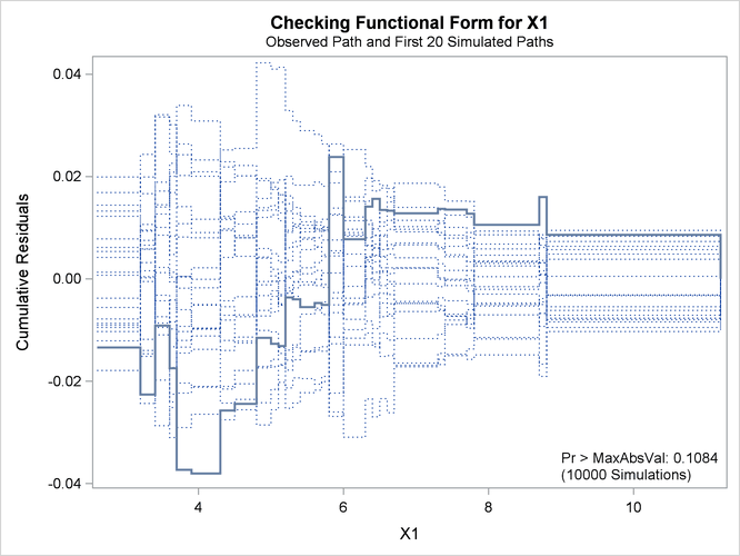
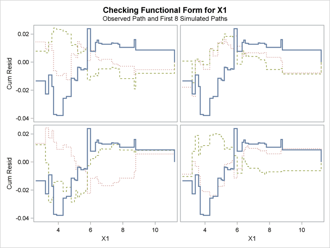
See Lin, Wei, and Ying (2002) for details about model assessment that uses cumulative residual plots. The RESAMPLE= keyword specifies that a p-value be computed based on a sample of 10,000 simulated residual paths. A random number seed is specified by the SEED= keyword for reproducibility. If you do not specify the seed, one is derived from the time of day. The keyword CRPANEL specifies that the panel of four cumulative residual plots shown in Output 44.8.4 be created, each with two simulated paths. The single residual plot with 20 simulated paths in Output 44.8.3 is created by default.

To request these graphs, ODS Graphics must be enabled and you must specify the ASSESS statement. For general information about ODS Graphics, see Chapter 21: Statistical Graphics Using ODS. For specific information about the graphics available in the GENMOD procedure, see the section ODS Graphics.

Output 44.8.3: Cumulative Residual Plot for Linear X1 Fit

Output 44.8.4: Cumulative Residual Panel Plot for Linear X1 Fit

Output 44.8.5: Summary of Model Assessment

Assessment Summary
Assessment Variable	Maximum Absolute Value	Replications	Seed	Pr > MaxAbsVal
X1	0.0380	10000	603708000	0.1084

The p-value of 0.1084 reported on Output 44.8.3 and Output 44.8.5 suggests that a more adequate model might be possible. The observed cumulative residuals in Output 44.8.3 and Output 44.8.4, represented by the heavy lines, seem atypical of the simulated curves, represented by the light lines, reinforcing the conclusion that a more appropriate functional form for X1 is possible.

The cumulative residual plots in Output 44.8.6 provide guidance in determining a more appropriate functional form. The four curves were created from simple forms of model misspecification by using simulated data. The mean models of the data and the fitted model are shown in Table 44.19.

Output 44.8.6: Typical Cumulative Residual Patterns

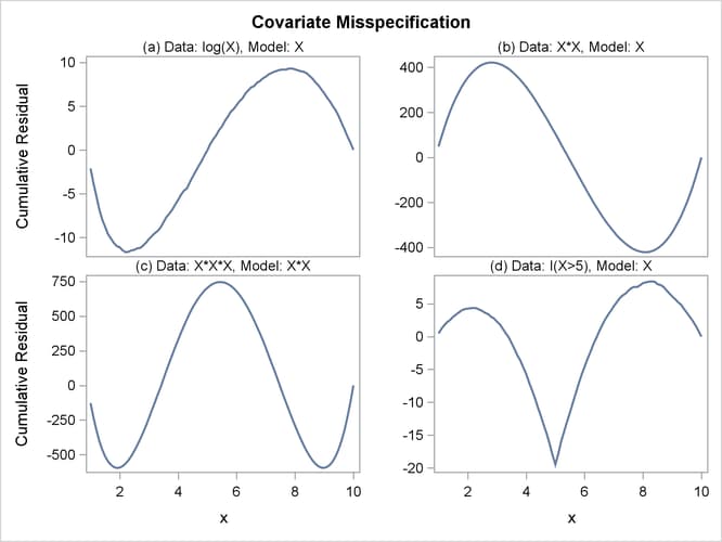
Table 44.19: Model Misspecifications

Plot	Data E(Y)	Fitted Model E(Y)
(a)	log(X)	X
(b)	$X + X^2$	X
(c)	$X + X^2 + X^3$	$X + X^2$
(d)	$I(X>5)$	X

The observed cumulative residual pattern in Output 44.8.3 and Output 44.8.4 most resembles the behavior of the curve in plot (a) of Output 44.8.6, indicating that log( $X_1$ ) might be a more appropriate term in the model than $X_1$ .

The following SAS statements fit a model with LogX1 in place of X1 and request a model assessment:

proc genmod data=Surg;
   model Y = LogX1 X2 X3 / scale=Pearson;
   assess var=(LogX1) / resample=10000
                        seed=603708000;
run;

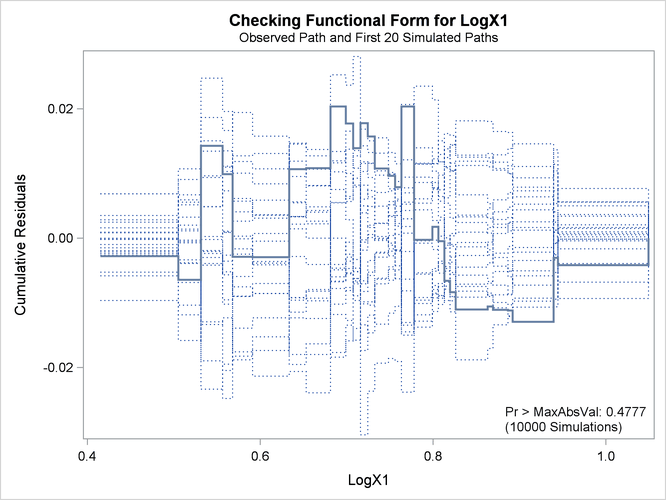
The revised model fit is shown in Output 44.8.7, the p-value from the simulation is 0.4777, and the cumulative residuals plotted in Output 44.8.8 show no systematic trend. The log transformation for X1 is more appropriate. Under the revised model, the p-values for testing the functional forms of X2 and X3 are 0.20 and 0.63, respectively; and the p-value for testing the linearity of the model is 0.65. Thus, the revised model seems reasonable.

Output 44.8.7: Multiple Regression Model with Log(X1)

The GENMOD Procedure

Analysis Of Maximum Likelihood Parameter Estimates
Parameter	DF	Estimate	Standard Error	Wald 95% Confidence Limits		Wald Chi-Square	Pr > ChiSq
Intercept	1	0.1844	0.0504	0.0857	0.2832	13.41	0.0003
LogX1	1	0.9121	0.0491	0.8158	1.0083	345.05	<.0001
X2	1	0.0095	0.0004	0.0088	0.0102	728.62	<.0001
X3	1	0.0096	0.0003	0.0090	0.0101	1139.73	<.0001
Scale	0	0.0434	0.0000	0.0434	0.0434

Note:

The scale parameter was estimated by the square root of Pearson's Chi-Square/DOF.

Output 44.8.8: Cumulative Residual Plot with Log(X1)