The GEE Procedure

Example 43.2 Log-Linear Model for Count Data
The following example demonstrates how you can fit a GEE model to count data. The data are analyzed by Diggle, Liang, and Zeger (1994). The response is the number of epileptic seizures, which was measured at the end of each of eight two-week treatment periods over sixteen weeks. The first eight weeks were the baseline period (during which no treatment was given), and the second eight weeks were the treatment period, during which patients received either a placebo or the drug progabide. The question of scientific interest is whether progabide is effective in reducing the rate of epileptic seizures.
The following DATA step creates the data set Seizure:
data Seizure;
   input ID Count Visit  Trt Age Weeks;
   datalines;
104 11 0 0 31 8
104 5 1 0 31 2
104 3 2 0 31 2
104 3 3 0 31 2
104 3 4 0 31 2
106 11 0 0 30 8

   ... more lines ...

236 12 0 1 37 8
236 1 1 1 37 2
236 4 2 1 37 2
236 3 3 1 37 2
236 2 4 1 37 2
;
The following DATA step creates a log time interval variable for use as an offset and an indicator variable for whether the observation is for a baseline measurement or a visit measurement. Patient 207 is deleted as an outlier, which was done in the Diggle et al. (2002) analysis:
data Seizure;
   set Seizure;
   if ID ne 207;
   if Visit = 0 then do;
      X1=0;
      Ltime = log(8);
   end;
   else do;
      X1=1;
      Ltime=log(2);
   end;
run;
Poisson regression is commonly used to model count data. In this example, the log-linear Poisson model is specified by  (the Poisson variance function) and a log link function,
![\[ \log (E(Y_{ij}))=\beta _{0}+x_{i1}\beta _{1}+x_{i2}\beta _{2}+ x_{i1}x_{i2}\beta _{3} + \log (t_{ij}) \]](images/statug_gee0196.png)
where
-
 number of epileptic seizures in interval j
-
 length of interval j
-
-
Because the visits represent repeated measurements, the responses from the same individual are correlated and inferences need
to take this into account. The correlations between the counts are modeled as  ,
,  (exchangeable correlations).
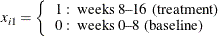
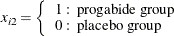
In this model, the regression parameters are interpreted in terms of the log seizure rate that is displayed in Table 43.14.
Table 43.14: Interpretation of Regression Parameters
|
Treatment |
Visit |
|
|---|---|---|
|
Placebo |
Baseline |
|
|
1–4 |
|
|
|
Progabide |
Baseline |
|
|
1–4 |
|


The difference between the log seizure rates in the pretreatment (baseline) period and the treatment periods is  for the placebo group and
  for the progabide group. A value of
  indicates a reduction in the seizure rate.
The following statements perform the analysis:
proc gee data = Seizure;
   class ID Visit;
   model Count = X1 Trt X1*Trt / dist=poisson link=log offset= Ltime;
   repeated subject = ID / within = Visit type=unstr covb corrw;
run;
In the MODEL statement, Count is the response variable, and X1, Trt, and the interaction X1*Trt are the explanatory variables. You request Poisson regression with the DIST=POISSON and the LINK=LOG options. The offset
variable is often used in Poisson regression to account for different exposures. In this case, the OFFSET= option specifies
Ltime as the offset variable representing different time intervals.
In the REPEATED statement, the SUBJECT= option indicates that the variable ID identifies the observations from a single cluster, and the TYPE=UNSTR option specifies the unstructured working correlation
structure. The CORRW option requests that the working correlation matrix be displayed.
The "Model Information" table that is displayed in Output 43.2.1 provides information about the specified model and the input data set.
Output 43.2.1: Model Information
Output 43.2.2 displays general information about the GEE model analysis.
Output 43.2.2: GEE Model Information
Output 43.2.3 displays the parameter estimate covariance matrices, which are requested by the COVB option. Both model-based and empirical covariances are produced.
Output 43.2.3: Covariance Matrices of Parameter Estimate
The exchangeable working correlation matrix is displayed in Output 43.2.4. It shows that there are noticeable correlations among the respective visits.
Output 43.2.4: Working Correlation Matrix
The parameter estimates table, shown in Output 43.2.5, contains parameter estimates, standard errors, confidence intervals, Z scores, and p-values for the parameter estimates. Empirical standard error estimates are used in this table.
Output 43.2.5: Parameter Estimates Table
| Parameter Estimates for Response Model | ||||||
|---|---|---|---|---|---|---|
| with Empirical Standard Error Estimates | ||||||
| Parameter | Estimate | Standard Error |
95% Confidence Limits | Z | Pr > |Z| | |
| Intercept | 1.3309 | 0.1612 | 1.0151 | 1.6468 | 8.26 | <.0001 |
| X1 | 0.1128 | 0.0927 | -0.0689 | 0.2945 | 1.22 | 0.2237 |
| Trt | -0.1034 | 0.1960 | -0.4875 | 0.2807 | -0.53 | 0.5978 |
| X1*Trt | -0.3162 | 0.1496 | -0.6093 | -0.0231 | -2.11 | 0.0345 |
The estimate of  is –0.3162, which indicates that progabide is effective in reducing the rate of epileptic seizures.
Model fit criteria for the model are displayed in Output 43.2.6. These criteria are used in selecting regression models and working correlations.