The GEE Procedure

Generalized Estimating Equations
The marginal model is commonly used in analyzing longitudinal data when the population-averaged effect is of interest. To estimate the regression parameters in the marginal model, Liang and Zeger (1986) proposed the generalized estimating equations method, which is widely used.
Suppose  , represent the jth response of the ith subject, which has a vector of covariates
  . There are
  measurements on subject i, and the maximum number of measurements per subject is T.
Suppose the responses of the ith subject be ![$\mb{Y}_{i}=[y_{i1}, \ldots , y_{i n_ i}]^{\prime }$](images/statug_gee0029.png) with corresponding means
with corresponding means ![$\bmu _{i}=[\mu _{i1}, \ldots , \mu _{i n_ i}]^{\prime }$](images/statug_gee0030.png) . For generalized linear models, the marginal mean
. For generalized linear models, the marginal mean  of the response
  is related to a linear predictor through a link function
  , and the variance of depends on the mean through a variance function
  .
.
An estimate of the parameter  in the marginal model can be obtained by solving the generalized estimating equations,
![\[ \mb{S}(\bbeta ) = \sum _{i=1}^ K \frac{\partial \bmu _{i}^{\prime }}{\partial \bbeta } \mb{V}_{i}^{-1} (\mb{Y}_{i}-\bmu _{i}(\bbeta )) = \mb{0} \]](images/statug_gee0036.png)
where  is the working covariance matrix of
  .
.
Only the mean and the covariance of are required in the GEE method; a full specification of the joint distribution of the correlated responses is not needed.
This is particularly convenient because the joint distribution for noncontinuous responses involves high-order associations
and is complicated to specify. Moreover, the regression parameter estimates are consistent even when the working covariance
is incorrectly specified. Because of these properties, the GEE method is popular in situations where the marginal effect is
of interest and the responses are not continuous. However, the GEE approach can lead to biased estimates when missing responses
depend on previous responses. The weighted GEE method, which is described in the section Weighted Generalized Estimating Equations under the MAR Assumption, can provide unbiased estimates.
Working Correlation Matrix
Suppose  is an
is an  "working" correlation matrix that is fully specified by the vector of parameters
  . The covariance matrix of is modeled as
![\[ \mb{V}_{i} = \phi \mb{A}_ i^{\frac{1}{2}} \mb{W}_ i^{-\frac{1}{2}} \mb{R}(\balpha ) \mb{W}_ i^{-\frac{1}{2}} \mb{A}_ i^{\frac{1}{2}} \]](images/statug_gee0042.png)
where  is an diagonal matrix whose jth diagonal element is and
  is an diagonal matrix whose jth diagonal is
  , where is a weight variable that is specified in the WEIGHT statement. If there is no WEIGHT statement,
  for all i and j. If is the true correlation matrix of , then is the true covariance matrix of .
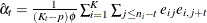
In practice, the working correlation matrix is usually unknown and must be estimated. It is estimated in the iterative fitting
process by using the current value of the parameter vector to compute appropriate functions of the Pearson residual:
![\[ e_{ij}=\frac{y_{ij}-\mu _{ij}}{\sqrt {v(\mu _{ij})/w_{ij}}} \]](images/statug_gee0047.png)
If you specify the working correlation matrix as  , which is the identity matrix, the GEE reduces to the independence estimating equation.
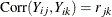
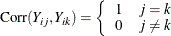
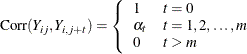
Table 43.11 shows the working correlation structures that are supported by the GEE procedure and the estimators that are used to estimate the working correlations.
Table 43.11: Working Correlation Structures and Estimators
|
Working Correlation Structure |
Estimator |
|---|---|
|
Fixed |
|
|
|
The working correlation is not estimated in this case. |
|
Independent |
|
|
|
The working correlation is not estimated in this case. |
|
m-dependent |
|
|
|
|
|
Exchangeable |
|
|
|
|
|
Unstructured |
|
|
|
|
|
Autoregressive AR(1) |
|
|
|
|


Dispersion Parameter
The dispersion parameter  is estimated by
![\[ \hat{\phi } = \frac{1}{N-p} \sum _{i=1}^ K \sum _{j=1}^{n_ i} e_{ij}^2 \]](images/statug_gee0066.png)
where  is the total number of measurements and p is the number of regression parameters.
The square root of  is reported by PROC GEE as the scale parameter in the "Parameter Estimates for Response Model with Model-Based Standard Error"
output table. If a fixed scale parameter is specified by using the NOSCALE option in the MODEL statement, then the fixed value
is used in estimating the model-based covariance matrix and standard errors.
is reported by PROC GEE as the scale parameter in the "Parameter Estimates for Response Model with Model-Based Standard Error"
output table. If a fixed scale parameter is specified by using the NOSCALE option in the MODEL statement, then the fixed value
is used in estimating the model-based covariance matrix and standard errors.
Quasi-likelihood Information Criterion
The quasi-likelihood information criterion (QIC) was developed by Pan (2001) as a modification of Akaike’s information criterion (AIC) to apply to models fit by the GEE approach.
Define the quasi-likelihood under the independent working correlation assumption, evaluated with the parameter estimates under the working correlation of interest as
![\[ Q(\hat{\bbeta }(R), \phi ) = \sum _{i=1}^ K\sum _{j=1}^{n_ i} Q(\hat{\bbeta }(R), \phi ; (Y_{ij}, \mb{X}_{ij})) \]](images/statug_gee0069.png)
where the quasi-likelihood contribution of the jth observation in the ith cluster is defined in the section Quasi-likelihood Functions and  are the parameter estimates that are obtained by using the GEE approach with the working correlation of interest R.
QIC is defined as
![\[ \mr{QIC}(R) = -2Q(\hat{\bbeta }(R), \phi ) + 2\mr{trace}(\hat{\Omega }_ I\hat{V}_ R) \]](images/statug_gee0071.png)
where  is the robust covariance estimate and
  is the inverse of the model-based covariance estimate under the independent working correlation assumption, evaluated at
, which are the parameter estimates that are obtained by using the GEE approach with the working correlation of interest R.
is the inverse of the model-based covariance estimate under the independent working correlation assumption, evaluated at
, which are the parameter estimates that are obtained by using the GEE approach with the working correlation of interest R.
PROC GEE also computes an approximation to  , which is defined by Pan (2001) as
![\[ \mr{QIC}_ u(R) = -2Q(\hat{\bbeta }(R), \phi ) + 2p \]](images/statug_gee0075.png)
where p is the number of regression parameters.
Pan (2001) notes that QIC is appropriate for selecting regression models and working correlations, whereas  is appropriate only for selecting regression models.
Quasi-likelihood Functions
See McCullagh and Nelder (1989) and Hardin and Hilbe (2003) for discussions of quasi-likelihood functions. The contribution of observation j in cluster i to the quasi-likelihood function that is evaluated at the regression parameters is expressed by  , where
  is defined in the following list. These definitions are used in the computation of the quasi-likelihood information criteria
(QIC) for goodness of fit of models that are fit by the GEE approach. The are prior weights, if any, that are specified in the WEIGHT or FREQ statement. Note that the definition of the quasi-likelihood
for the negative binomial differs from that given in McCullagh and Nelder (1989). The definition used here allows the negative binomial quasi-likelihood to approach the Poisson as
is defined in the following list. These definitions are used in the computation of the quasi-likelihood information criteria
(QIC) for goodness of fit of models that are fit by the GEE approach. The are prior weights, if any, that are specified in the WEIGHT or FREQ statement. Note that the definition of the quasi-likelihood
for the negative binomial differs from that given in McCullagh and Nelder (1989). The definition used here allows the negative binomial quasi-likelihood to approach the Poisson as  .
.
-
Normal:
![\[ Q_{ij} = -\frac{1}{2} w_{ij}(y_{ij}-\mu _{ij})^2 \]](images/statug_gee0080.png)
-
Inverse Gaussian:
![\[ Q_{ij} = \frac{w_{ij}(\mu _{ij} - .5y_{ij})}{\mu _{ij}^2 } \]](images/statug_gee0081.png)
-
Gamma:
![\[ Q_{ij} = -w_{ij}\left[ \frac{y_{ij}}{\mu _{ij}} + \log (\mu _{ij}) \right] \]](images/statug_gee0082.png)
-
Negative binomial:
![\[ Q_{ij} = w_{ij}\left[ \log \Gamma \left( y_{ij} + \frac{1}{k}\right) - \log \Gamma \left(\frac{1}{k}\right) + y_{ij}\log \left(\frac{k\mu _{ij}}{1+k\mu _{ij}}\right) + \frac{1}{k}\log \left(\frac{1}{1+k\mu _{ij}}\right)\right] \]](images/statug_gee0083.png)
-
Poisson:
![\[ Q_{ij} = w_{ij}(y_{ij} \log (\mu _{ij}) - \mu _{ij} ) \]](images/statug_gee0084.png)
-
Binomial:
![\[ Q_{ij} = w_{ij}[r_{ij} \log (p_{ij}) + (n_{ij}-r_{ij}) \log (1-p_{ij})] \]](images/statug_gee0085.png)
-
Multinomial (s categories):
![\[ Q_{ij} = w_{ij}\sum _{k=1}^ s y_{ijk}\log (\mu _{ijk}) \]](images/statug_gee0086.png)