The BCHOICE Procedure (Experimental)

This example uses a standard logit model in which the error component, ![]() , is independently and identically distributed (iid) with the Type I extreme-value distribution,
, is independently and identically distributed (iid) with the Type I extreme-value distribution, ![]() . This assumption provides a convenient form for the choice probability (McFadden, 1974):
. This assumption provides a convenient form for the choice probability (McFadden, 1974):
The likelihood is formed by the product of the N independent multinomial distributions:
Suppose you want a normal prior on ![]()
where ![]() is the identity matrix and c is a scalar. c is often set to be large for a noninformative prior.
is the identity matrix and c is a scalar. c is often set to be large for a noninformative prior.
The posterior density of the parameter ![]() is
is
PROC BCHOICE obtains samples from the posterior distribution, produces summary and diagnostic statistics, and saves the posterior samples in an output data set that can be used for further analysis.
In this example (Kuhfeld, 2010), each of 10 subjects is presented with eight different chocolate candies and asked to choose one. The eight candies consist
of the ![]() combinations of dark or milk chocolate, soft or chewy center, and nuts or no nuts. Each subject sees all eight alternatives
and makes one choice. Experimental choice data such as these are usually analyzed by using a multinomial logit model.
combinations of dark or milk chocolate, soft or chewy center, and nuts or no nuts. Each subject sees all eight alternatives
and makes one choice. Experimental choice data such as these are usually analyzed by using a multinomial logit model.
The following statements read the data:
title 'Conjoint Analysis of Chocolate Candies';

data Chocs;
   input Subj Choice Dark Soft Nuts;
   datalines;
1 0 0 0 0
1 0 0 0 1
1 0 0 1 0
1 0 0 1 1
1 1 1 0 0
1 0 1 0 1

   ... more lines ...

10 0 1 0 0
10 1 1 0 1
10 0 1 1 0
10 0 1 1 1
;
proc print data=Chocs (obs=16);
   by Subj;
   id Subj;
run;
The data for the first two subjects are shown in Figure 27.1.
Figure 27.1: Data for the First Two Subjects
| Conjoint Analysis of Chocolate Candies |
| Subj | Choice | Dark | Soft | Nuts |
|---|---|---|---|---|
| 1 | 0 | 0 | 0 | 0 |
| 0 | 0 | 0 | 1 | |
| 0 | 0 | 1 | 0 | |
| 0 | 0 | 1 | 1 | |
| 1 | 1 | 0 | 0 | |
| 0 | 1 | 0 | 1 | |
| 0 | 1 | 1 | 0 | |
| 0 | 1 | 1 | 1 |
| Subj | Choice | Dark | Soft | Nuts |
|---|---|---|---|---|
| 2 | 0 | 0 | 0 | 0 |
| 0 | 0 | 0 | 1 | |
| 0 | 0 | 1 | 0 | |
| 0 | 0 | 1 | 1 | |
| 0 | 1 | 0 | 0 | |
| 1 | 1 | 0 | 1 | |
| 0 | 1 | 1 | 0 | |
| 0 | 1 | 1 | 1 |
The data set contains 10 subjects and 80 observation lines. Each line of the data represents one alternative in the choice
set for each subject. It is required that the response variable, which is Choice in this study, indicate the chosen alternative by the value 1 and the unchosen alternatives by the value 0. Dark is 1 for dark chocolate and 0 for milk chocolate; Soft is 1 for soft center and 0 for chewy center; Nuts is 1 if the candy contains nuts and 0 if it does not contain nuts. In this example, subject 1 chose the fifth alternative
(Choice=1, which is Dark/Chewy/No Nuts) among the eight alternatives in the choice set. All the chosen and unchosen alternatives
must appear in the data set. If you have choice data in which all alternatives appear on one line, then you must rearrange
the data in the correct form (that is, the data must contain one observation line for each alternative of each choice set
for each subject).
The following statements fit a multinomial logit model:
ods graphics on;
proc bchoice data=Chocs outpost=Bsamp nmc=10000 thin=2 diag=(AutoCorr
     ESS MCSE) seed=124;
   class Dark(ref='0') Soft(ref='0') Nuts(ref='0') Subj;
   model Choice = Dark Soft Nuts / choiceset=(Subj) cprior=normal(var=1000);
run;
The ODS GRAPHICS ON statement invokes the ODS Graphics environment and displays the diagnostic plots, such as the trace and autocorrelation function plots of the posterior samples. For more information about ODS, see Chapter 21: Statistical Graphics Using ODS.
The PROC BCHOICE statement invokes the procedure, and the DATA= option specifies the input data set Chocs. The OUTPOST= requests an output data set called Bsamp to contain all the posterior samples. The NMC= option specifies the number of posterior simulation iterations. The THIN= option controls the thinning of the Markov chain and specifies that one of every two samples be kept. Thinning is often used
to reduce correlation among posterior sample draws. In this example, 5,000 simulated values are saved in the Bsamp data set. The DIAG=(AUTOCORR ESS MCSE) option requests that three convergence diagnostics be output to help determine whether the chain has converged:
the autocorrelations, effective sample sizes, and Monte Carlo standard errors. The SEED= option specifies a seed for the random number generator, which guarantees the reproducibility of the random stream.
The CLASS statement names the classification variables to be used in the model. The CLASS statement must precede the MODEL statement (as it must in most other SAS procedures). The REF= option specifies the reference level.
The MODEL statement is required; it defines the dependent variable (![]() ) and independent variables (
) and independent variables (![]() ). To the left of the equal sign in the MODEL statement, you specify the dependent variable that indicates which alternatives are chosen and which ones are not chosen.
The dependent variable
). To the left of the equal sign in the MODEL statement, you specify the dependent variable that indicates which alternatives are chosen and which ones are not chosen.
The dependent variable Choice has values 1 (chosen) and 0 (unchosen). You specify the independent variables after the equal sign. The independent variables
often indicate attributes or characteristics of the alternatives in the choice set, such as Dark, Soft, and Nuts in this example. The CHOICESET= option specifies how a choice set is defined. In this example, CHOICESET=(Subj) because there is one and only one choice
set per subject. The variable that you specify in the CHOICESET= option must be a classification variable that appears in the CLASS statement. You should always use the CHOICESET= option to define the choice set.
The first table that PROC BCHOICE produces is the “Model Information” table, as shown in Figure 27.2. This table displays basic information about the analysis, such as the name of the input data set, response variable, model type, sampling algorithm, burn-in size, simulation size, thinning number, and random number seed. The random number seed initializes the random number generators. If you repeat the analysis and use the same seed, you get an identical stream of random numbers.
Figure 27.2: Model Information
| Model Information | |
|---|---|
| Data Set | WORK.CHOCS |
| Response Variable | Choice |
| Type of Model | Logit |
| Fixed Effects Included | Yes |
| Random Effects Included | No |
| Sampling Algorithm | Gamerman Metropolis |
| Burn-In Size | 500 |
| Simulation Size | 10000 |
| Thinning | 2 |
| Random Number Seed | 124 |
| Number of Threads | 1 |
The “Choice Sets Summary” table is displayed by default and should be used to check the data entry. In this case, there are 10 choice sets, one for each subject. All 10 choice sets display the same pattern: they have eight total alternatives, one of which is chosen and seven of which are unchosen. PROC BCHOICE requires that all choice sets have a pattern of the same number of total alternatives, one of which is the chosen alternative. If there is more than one pattern among the choice sets (for example, some choice sets have nine alternatives or some subjects chose two alternatives), a warning message appears in the SAS log and those invalid choice sets are excluded from analysis.
Figure 27.3: Choice Sets Summary
| Choice Sets Summary | ||||
|---|---|---|---|---|
| Pattern | Choice Sets | Total Alternatives |
Chosen Alternatives |
Not Chosen |
| 1 | 10 | 8 | 1 | 7 |
The next table is the “Number of Observations” table, as shown in Figure 27.4. This table lists the number of observations that are read from the DATA= data set and the number of nonmissing and valid observations that are used in the analysis. PROC BCHOICE does not impute missing values. If any missing value is encountered in a row of the DATA= data set, PROC BCHOICE skips that row and moves on to read the next row. If the missing value causes the corresponding choice set to have a pattern different from that of the rest of the choice sets, the entire choice set is discarded from analysis. In this example, all 80 observations are used.
Figure 27.4: Number of Observations
| Number of Observations | |
|---|---|
| Number of Observations Read | 80 |
| Number of Observations Used | 80 |
PROC BCHOICE reports posterior summary statistics (posterior means, standard deviations, and HPD intervals) for each parameter, as shown in Figure 27.5. For more information about posterior statistics, see the section Summary Statistics.
Figure 27.5: PROC BCHOICE Posterior Summary Statistics
| Posterior Summaries and Intervals | |||||
|---|---|---|---|---|---|
| Parameter | N | Mean | Standard Deviation |
95% HPD Interval | |
| Dark 1 | 5000 | 1.5308 | 0.7943 | 0.1848 | 3.2412 |
| Soft 1 | 5000 | -2.4312 | 0.9792 | -4.4882 | -0.8125 |
| Nuts 1 | 5000 | 0.9671 | 0.7454 | -0.3255 | 2.6675 |
Before you examine the posterior summary statistics and try to draw any conclusions, you might want to verify that the simulation has converged. Convergence diagnostics are essential to inferring from simulations that are based on Markov chains. If the Markov chain has not converged, all conclusions that are based on the samples might be misleading. PROC BCHOICE computes the effective sample size by default. There are a number of other convergence diagnostics to help you determine whether the chain has converged: the Monte Carlo standard errors, the autocorrelations at selected lags, and so on. These statistics are shown in Figure 27.6. For details and interpretations of these diagnostics, see the section Assessing Markov Chain Convergence.
The “Posterior Autocorrelations” table shows that the autocorrelations among posterior samples reduce quickly. The “Effective Sample Sizes” table reports the number of effective sample sizes of the Markov chain. The “Monte Carlo Standard Errors” table indicates that the standard errors of the mean estimates for each of the variables are relatively small with respect to the posterior standard deviations. The values in the MCSE/SD column (ratios of the standard errors and the standard deviations) are small. This means that only a fraction of the posterior variability is caused by the simulation.
Figure 27.6: PROC BCHOICE Convergence Diagnostics
| Posterior Autocorrelations | ||||
|---|---|---|---|---|
| Parameter | Lag 1 | Lag 5 | Lag 10 | Lag 50 |
| Dark 1 | 0.4495 | 0.1427 | 0.0603 | -0.0095 |
| Soft 1 | 0.5389 | 0.1518 | 0.0730 | 0.0449 |
| Nuts 1 | 0.4136 | 0.1473 | 0.0259 | -0.0264 |
| Effective Sample Sizes | |||
|---|---|---|---|
| Parameter | ESS | Autocorrelation Time |
Efficiency |
| Dark 1 | 1078.4 | 4.6365 | 0.2157 |
| Soft 1 | 904.9 | 5.5253 | 0.1810 |
| Nuts 1 | 1161.6 | 4.3043 | 0.2323 |
| Monte Carlo Standard Errors | |||
|---|---|---|---|
| Parameter | MCSE | Standard Deviation |
MCSE/SD |
| Dark 1 | 0.0242 | 0.7943 | 0.0305 |
| Soft 1 | 0.0326 | 0.9792 | 0.0332 |
| Nuts 1 | 0.0219 | 0.7454 | 0.0293 |
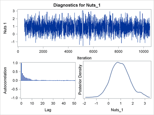
PROC BCHOICE produces a number of graphs, shown in Figure 27.7, which also aid convergence diagnostic checks. The trace plots have two important aspects to examine. First, you want to check whether the mean of the Markov chain has stabilized and appears constant over the graph. Second, you want to check whether the chain has good mixing and is “dense,” in the sense that it quickly traverses the support of the distribution to explore both the tails and the mode areas efficiently. The plots show that the chains appear to have reached their stationary distributions.
Next, you want to examine the autocorrelation plots, which indicate the degree of autocorrelation for each of the posterior samples. High correlations usually imply slow mixing. Finally, the kernel density plots estimate the posterior marginal distributions for each parameter.


Because the chains have converged, you can go back to the posterior summary table for results and conclusions. As seen in Figure 27.5, the part-worth for dark chocolate is 1.5 and the part-worth for milk chocolate (base category) is structural 0; the part-worth for soft center is –2.4 and the part-worth for chewy center is structural 0; the part-worth for containing nuts is 1.0 and the part-worth for no nuts is structural 0. A positive part-worth implies being more favorable. Hence, dark chocolate is preferred over milk chocolate, soft centers are less popular than chewy centers, and candies with nuts are more popular than candies without nuts.