The BCHOICE Procedure (Experimental)

Choice models that have random effects (or random coefficients) provide solutions to create individual-level or group-specific utilities. Because people have different preferences, it can be misleading to roll the whole sample together into a single set of utilities. The desire to account for individual differences, instead of treating all respondents alike, provides challenges in marketing research. For logit models that have random effects, using frequentist methods to optimize of the likelihood function can be numerically difficult. Bayesian methods are ideally suited for analysis with random effects.
Choice models that have random effects generalize the standard choice models to incorporate individual-level effects. Let
the utility that individual i obtains from alternative j in choice situation t (![]() ) be
) be
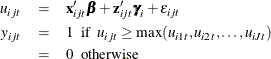
where ![]() is the observed choice for individual i and alternative j in choice situation t;
is the observed choice for individual i and alternative j in choice situation t; ![]() is the fixed design vector for individual i and alternative j in choice situation t;
is the fixed design vector for individual i and alternative j in choice situation t; ![]() are the fixed coefficients;
are the fixed coefficients; ![]() is the random design vector for individual i and alternative j in choice situation t; and
is the random design vector for individual i and alternative j in choice situation t; and ![]() are the random coefficients for individual i corresponding to
are the random coefficients for individual i corresponding to ![]() .
.
It is assumed that each ![]() is drawn from a superpopulation and that this superpopulation is normal,
is drawn from a superpopulation and that this superpopulation is normal, ![]() . An additional stage is added to the model in which a prior for
. An additional stage is added to the model in which a prior for ![]() is specified:
is specified:
The covariance matrix ![]() characterizes the extent of unobserved heterogeneity among individuals. Large diagonal elements of
characterizes the extent of unobserved heterogeneity among individuals. Large diagonal elements of ![]() indicate substantial heterogeneity in part-worths. Off-diagonal elements indicate patterns in the evaluation of attribute
levels.
indicate substantial heterogeneity in part-worths. Off-diagonal elements indicate patterns in the evaluation of attribute
levels.
Consider a study that estimates the market demand for kitchen trash cans (Rossi, 2013). There are four attributes, and each has two levels: touchless opening (Yes/No), material (Steel/Plastic), automatic trash
bag replacement (Yes/No), and price (![]() 40). The number of all possible hypothetical types of trash cans is
40). The number of all possible hypothetical types of trash cans is ![]() . Including more attributes and more levels can easily become unmanageable. The study uses a fractional factorial design,
in which the first three factors are set up to be a full factorial design and the fourth is generated as the product of the
first three. This design confounds the three-way interaction with the effect of the fourth factor, shown in Table 27.1.
. Including more attributes and more levels can easily become unmanageable. The study uses a fractional factorial design,
in which the first three factors are set up to be a full factorial design and the fourth is generated as the product of the
first three. This design confounds the three-way interaction with the effect of the fourth factor, shown in Table 27.1.
Table 27.1: Design for the Trash Can Study
|
Obs |
Touchless |
Steel |
AutoBag |
Price80 |
|
1 |
–1 |
–1 |
–1 |
–1 |
|
2 |
–1 |
–1 |
1 |
1 |
|
3 |
–1 |
1 |
–1 |
1 |
|
4 |
–1 |
1 |
1 |
–1 |
|
5 |
1 |
–1 |
–1 |
1 |
|
6 |
1 |
–1 |
1 |
–1 |
|
7 |
1 |
1 |
–1 |
–1 |
|
8 |
1 |
1 |
1 |
1 |
In Table 27.1, 1 means “Yes” and –1 means “No.” This is a balanced design, in which each level appears the same number of times. This study assigns only two alternatives to a choice set by randomly sampling two rows from the previous table and giving each individual 10 choice sets (or choice tasks) to pick from. For more information about how to design a choice model efficiently, see Kuhfeld (2010).
Data were obtained by enrolling 104 people and assigning 10 choice tasks to each of them: for each task, the participants stated their preference between two types of trash cans. The following steps read in the data:
data Trashcan;
   input ID Task Choice Index Touchless Steel AutoBag Price80 @@;
   datalines;
1 1 1 1 0 1 1 0 1 1 0 2 1 1 0 0 1 2 0 1 0 0 0 0 1 2 1 2 1 1 1 1 1 3 0 1
0 0 0 0 1 3 1 2 1 1 0 0 1 4 0 1 0 1 0 1 1 4 1 2 1 0 0 1 1 5 1 1 0 1 1 0
1 5 0 2 1 0 0 1 1 6 0 1 0 0 1 1 1 6 1 2 1 1 1 1 1 7 0 1 1 0 0 1 1 7 1 2
1 1 0 0 1 8 0 1 0 0 1 1 1 8 1 2 0 1 1 0 1 9 1 1 0 0 1 1 1 9 0 2 1 0 0 1
1 10 0 1 0 1 1 0 1 10 1 2 1 0 1 0 2 1 1 1 0 1 1 0 2 1 0 2 1 1 0 0 2 2 0
1 0 0 0 0 2 2 1 2 1 1 1 1 2 3 0 1 0 0 0 0 2 3 1 2 1 1 0 0 2 4 0 1 0 1 0
1 2 4 1 2 1 0 0 1 2 5 1 1 0 1 1 0 2 5 0 2 1 0 0 1 2 6 1 1 0 0 1 1 2 6 0
2 1 1 1 1 2 7 1 1 1 0 0 1 2 7 0 2 1 1 0 0 2 8 1 1 0 0 1 1 2 8 0 2 0 1 1
0 2 9 1 1 0 0 1 1 2 9 0 2 1 0 0 1 2 10 1 1 0 1 1 0 2 10 0 2 1 0 1 0 3 1

   ... more lines ...

2 1 2 1 1 1 1 104 3 0 1 0 0 0 0 104 3 1 2 1 1 0 0 104 4 0 1 0 1 0 1 104
4 1 2 1 0 0 1 104 5 1 1 0 1 1 0 104 5 0 2 1 0 0 1 104 6 0 1 0 0 1 1 104
6 1 2 1 1 1 1 104 7 0 1 1 0 0 1 104 7 1 2 1 1 0 0 104 8 0 1 0 0 1 1 104
8 1 2 0 1 1 0 104 9 0 1 0 0 1 1 104 9 1 2 1 0 0 1 104 10 0 1 0 1 1 0 104
10 1 2 1 0 1 0
;
proc print data=Trashcan (obs=20);
   by ID Task;
   id ID Task;
run;
The data for the first four choice tasks are shown in Figure 27.8.
Figure 27.8: Data for the First Four Choice Tasks
| ID | Task | Choice | Index | Touchless | Steel | AutoBag | Price80 |
|---|---|---|---|---|---|---|---|
| 1 | 1 | 1 | 1 | 0 | 1 | 1 | 0 |
| 0 | 2 | 1 | 1 | 0 | 0 |
| ID | Task | Choice | Index | Touchless | Steel | AutoBag | Price80 |
|---|---|---|---|---|---|---|---|
| 1 | 2 | 0 | 1 | 0 | 0 | 0 | 0 |
| 1 | 2 | 1 | 1 | 1 | 1 |
| ID | Task | Choice | Index | Touchless | Steel | AutoBag | Price80 |
|---|---|---|---|---|---|---|---|
| 1 | 3 | 0 | 1 | 0 | 0 | 0 | 0 |
| 1 | 2 | 1 | 1 | 0 | 0 |
| ID | Task | Choice | Index | Touchless | Steel | AutoBag | Price80 |
|---|---|---|---|---|---|---|---|
| 1 | 4 | 0 | 1 | 0 | 1 | 0 | 1 |
| 1 | 2 | 1 | 0 | 0 | 1 |
In the data, ID is the individual’s ID number, and Task indexes the number of choice tasks. The response is Choice, which states each individual’s choice for each choice task. Touchless, Steel, AutoBag, and Price80 are the attribute variables; for each of them, 1 means “Yes” and 0 means “No.” In the data, 0 replaces the –1 values that are shown in the design matrix in Table 27.1.
The following statements fit a logit model with random effects:
proc bchoice data=Trashcan seed=123 nmc=20000 thin=4;
   class ID Task;
   model Choice = Touchless Steel AutoBag Price80 / choiceset=(ID Task);
   random Touchless Steel AutoBag Price80 / sub=ID monitor=(1 to 5) type=un;
run;
The choice set is specified by ID (which identifies the participants) and by Task (which identifies each of the 10 choice tasks that are assigned to each participant). The variables ID and Task are needed in the CLASS statement because they define the choice set in the MODEL statement.
In addition to the MODEL statement for fixed effects, the RANDOM statement is added for random effects. Note that Touchless, Steel, AutoBag, and Price80 are listed as both fixed and random effects, so that their average part-worth values in the population are estimated via
fixed effects and the deviation from the overall mean for each individual is presented through random effects. The SUB=ID argument in the RANDOM statement defines ID as a subject index for the random effects grouping, so that each person with a different ID has his or her own random effects. The MONITOR option requests the production of the individual-level random-effects parameter estimates, and the MONITOR=(1 to 5) option requests the random-effects parameter estimates for the first five subjects, (By default, PROC BCHOICE does
not output results for any individual-level random-effects parameters.) The TYPE=UN option in the RANDOM statement specifies an unstructured covariance matrix for the random effects. The unstructured type provides a mechanism
for estimating the correlation between the random effects. The TYPE=VC (variance components) option, which is the default structure, models a different variance component for each random effect.
Summary statistics for the fixed coefficients (![]() ), the covariance of the random coefficients (
), the covariance of the random coefficients (![]() ), and the random coefficients (
), and the random coefficients (![]() ) for the first five individuals are shown in Figure 27.9.
) for the first five individuals are shown in Figure 27.9.
Figure 27.9: Posterior Summary Statistics
| Posterior Summaries and Intervals | ||||||
|---|---|---|---|---|---|---|
| Parameter | Subject | N | Mean | Standard Deviation |
95% HPD Interval | |
| Touchless | 5000 | 1.7432 | 0.2758 | 1.2225 | 2.2974 | |
| Steel | 5000 | 1.0366 | 0.2749 | 0.5043 | 1.5951 | |
| AutoBag | 5000 | 2.1776 | 0.3556 | 1.4799 | 2.8655 | |
| Price80 | 5000 | -4.6574 | 0.6732 | -5.9315 | -3.3896 | |
| RECov Touchless, Touchless | 5000 | 3.2690 | 1.0960 | 1.4597 | 5.4938 | |
| RECov Steel, Touchless | 5000 | -0.5786 | 0.9401 | -2.6960 | 1.1540 | |
| RECov Steel, Steel | 5000 | 2.7386 | 0.9952 | 1.1160 | 4.7779 | |
| RECov AutoBag, Touchless | 5000 | -0.6080 | 0.8920 | -2.3911 | 1.2471 | |
| RECov AutoBag, Steel | 5000 | -0.0456 | 0.7354 | -1.5824 | 1.3500 | |
| RECov AutoBag, AutoBag | 5000 | 3.6331 | 1.5755 | 0.8716 | 6.5751 | |
| RECov Price80, Touchless | 5000 | -1.4322 | 1.2425 | -4.0486 | 0.6300 | |
| RECov Price80, Steel | 5000 | -1.5099 | 1.2504 | -4.1057 | 0.7940 | |
| RECov Price80, AutoBag | 5000 | -2.3795 | 1.7869 | -5.8962 | 0.5972 | |
| RECov Price80, Price80 | 5000 | 7.9205 | 3.5695 | 2.3922 | 14.7155 | |
| Touchless | ID 1 | 5000 | 0.5492 | 1.0522 | -1.5118 | 2.6518 |
| Steel | ID 1 | 5000 | -0.3691 | 1.1114 | -2.7311 | 1.7119 |
| AutoBag | ID 1 | 5000 | 1.6954 | 1.4487 | -0.8981 | 4.5846 |
| Price80 | ID 1 | 5000 | -0.7483 | 2.3010 | -5.2892 | 3.6146 |
| Touchless | ID 2 | 5000 | -1.8146 | 0.9255 | -3.6760 | 0.0196 |
| Steel | ID 2 | 5000 | -1.4133 | 0.8567 | -3.0222 | 0.3404 |
| AutoBag | ID 2 | 5000 | 0.4091 | 1.3343 | -2.1911 | 2.9911 |
| Price80 | ID 2 | 5000 | 4.6933 | 1.5455 | 1.8588 | 7.8627 |
| Touchless | ID 3 | 5000 | -0.7099 | 1.0230 | -2.7242 | 1.3434 |
| Steel | ID 3 | 5000 | 0.6959 | 1.0397 | -1.2993 | 2.7718 |
| AutoBag | ID 3 | 5000 | -1.9793 | 1.2506 | -4.3813 | 0.5263 |
| Price80 | ID 3 | 5000 | 3.8323 | 1.7134 | 0.3076 | 7.0044 |
| Touchless | ID 4 | 5000 | -0.6107 | 0.9869 | -2.5368 | 1.3259 |
| Steel | ID 4 | 5000 | 0.3235 | 1.0106 | -1.5620 | 2.3570 |
| AutoBag | ID 4 | 5000 | 1.0191 | 1.4644 | -1.5675 | 4.0437 |
| Price80 | ID 4 | 5000 | -1.8942 | 2.3716 | -6.8807 | 2.3238 |
| Touchless | ID 5 | 5000 | -1.3562 | 1.2145 | -3.7166 | 0.9827 |
| Steel | ID 5 | 5000 | 1.7447 | 1.2911 | -0.7051 | 4.1791 |
| AutoBag | ID 5 | 5000 | 1.1826 | 1.5781 | -1.8454 | 4.3037 |
| Price80 | ID 5 | 5000 | -0.3420 | 2.4111 | -4.9867 | 4.3344 |
The fixed effects (Touchless, Steel, AutoBag, and Price80) are shown in the first four rows. Across all the respondents in the data, the average part-worths for touchless opening,
steel material, and automatic trash bag replacement are all positive, indicating that most people favor those features; the
average part-worth for having to pay USD80 for a trash can instead of USD40 is negative (–4.7), which is very intuitive, because
spending more money is usually unfavorable.
The covariance estimate of the random coefficients (![]() ) is displayed by the parameters whose label begins with “RECov”:
) is displayed by the parameters whose label begins with “RECov”:
![\[ \hat{\bOmega }_{\bgamma } = \begin{pmatrix} 3.3 & . & . & . \\ -0.6 & 2.7 & . & . \\ -0.6 & -0.1 & 3.6 & . \\ -1.4 & -1.5 & -2.4 & 7.9 \end{pmatrix} \]](images/statug_bchoice0032.png)
where the dots refer to the corresponding elements in the lower part of the symmetric covariance matrix. The covariance estimate
of the random coefficients (![]() ) characterizes the variability of part-worths across respondents. Some of the diagonal elements of the matrix are large.
For example, the variance for price (labeled “RECov Price80, Price80”) is quite large, indicating substantial unexplained difference in response to price. Off-diagonal elements of the matrix
illustrate attribute levels that tend to be evaluated similarly (positive covariance) or differently (negative covariance)
across all the respondents. The covariances between each of the attributes (
) characterizes the variability of part-worths across respondents. Some of the diagonal elements of the matrix are large.
For example, the variance for price (labeled “RECov Price80, Price80”) is quite large, indicating substantial unexplained difference in response to price. Off-diagonal elements of the matrix
illustrate attribute levels that tend to be evaluated similarly (positive covariance) or differently (negative covariance)
across all the respondents. The covariances between each of the attributes (Touchless, Steel, and AutoBag) and Price80 are all negative, implying that the respondents who prefer some of the new features are those who are also unwilling to pay
a higher price for the trash can. Therefore, offering a discounted price might be a particularly effective method of introducing
the new features to customers.
The next set of parameters that are displayed are the estimates for the individual-level random effects for the first five respondents (see Figure 27.9). These estimates are the deviation from the overall means (which are estimated via the fixed effects). The part-worth for touchless opening for the first respondent (who is labeled “ID 1” in the Subject column) is 1.7 + 0.5 = 2.2.
Allenby and Rossi (1999) and Rossi, Allenby, and McCulloch (2005) propose a hierarchical Bayesian random-effects model that is set up in a different way such that there are no fixed effects but only random effects. For more information about this type of model, see the section Random Effects and a follow-up example in A Random-Effects-Only Logit Model.