Simulation-based Bayesian inference requires using simulated draws to summarize the posterior distribution or calculate any relevant quantities of interest. You need to treat the simulation draws with care. There are usually two issues. First, you have to decide whether the Markov chain has reached its stationary, or the desired posterior, distribution. Second, you have to determine the number of iterations to keep after the Markov chain has reached stationarity. Convergence diagnostics help to resolve these issues. Note that many diagnostic tools are designed to verify a necessary but not sufficient condition for convergence. There are no conclusive tests that can tell you when the Markov chain has converged to its stationary distribution. You should proceed with caution. Also, note that you should check the convergence of all parameters, and not just those of interest, before proceeding to make any inference. With some models, certain parameters can appear to have very good convergence behavior, but that could be misleading due to the slow convergence of other parameters. If some of the parameters have bad mixing, you cannot get accurate posterior inference for parameters that appear to have good mixing. See Cowles and Carlin (1996) and Brooks and Roberts (1998) for discussions about convergence diagnostics.
Trace plots of samples versus the simulation index can be very useful in assessing convergence. The trace tells you if the
chain has not yet converged to its stationary distribution—that is, if it needs a longer burn-in period. A trace can also
tell you whether the chain is mixing well. A chain might have reached stationarity if the distribution of points is not changing
as the chain progresses. The aspects of stationarity that are most recognizable from a trace plot are a relatively constant
mean and variance. A chain that mixes well traverses its posterior space rapidly, and it can jump from one remote region of
the posterior to another in relatively few steps. Figure 7.1 through Figure 7.4 display some typical features that you might see in trace plots. The traces are for a parameter called ![]() .
.
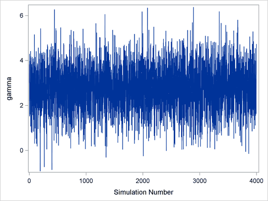
Figure 7.1 displays a “perfect” trace plot. Note that the center of the chain appears to be around the value 3, with very small fluctuations. This indicates that the chain could have reached the right distribution. The chain is mixing well; it is exploring the distribution by traversing to areas where its density is very low. You can conclude that the mixing is quite good here.
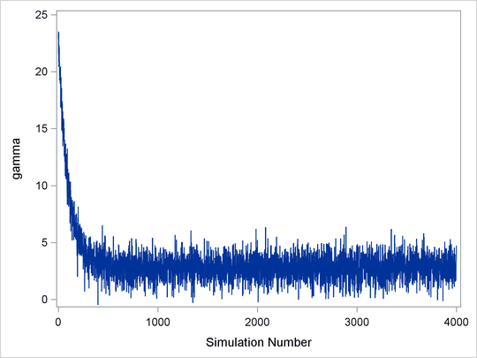
Figure 7.2 displays a trace plot for a chain that starts at a very remote initial value and makes its way to the targeting distribution. The first few hundred observations should be discarded. This chain appears to be mixing very well locally. It travels relatively quickly to the target distribution, reaching it in a few hundred iterations. If you have a chain that looks like this, you would want to increase the burn-in sample size. If you need to use this sample to make inferences, you would want to use only the samples toward the end of the chain.
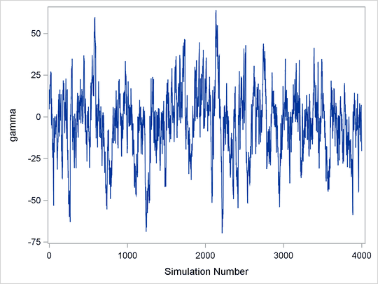
Figure 7.3 demonstrates marginal mixing. The chain is taking only small steps and does not traverse its distribution quickly. This type of trace plot is typically associated with high autocorrelation among the samples. To obtain a few thousand independent samples, you need to run the chain for much longer.
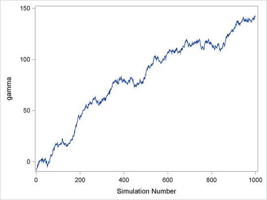
The trace plot shown in Figure 7.4 depicts a chain with serious problems. It is mixing very slowly, and it offers no evidence of convergence. You would want to try to improve the mixing of this chain. For example, you might consider reparameterizing your model on the log scale. Run the Markov chain for a long time to see where it goes. This type of chain is entirely unsuitable for making parameter inferences.
The Bayesian procedures include several statistical diagnostic tests that can help you assess Markov chain convergence. For a detailed description of each of the diagnostic tests, see the following subsections. Table 7.1 provides a summary of the diagnostic tests and their interpretations.
Table 7.1: Convergence Diagnostic Tests Available in the Bayesian Procedures
|
Name |
Description |
Interpretation of the Test |
|---|---|---|
|
Gelman-Rubin |
Uses parallel chains with dispersed initial values to test whether they all converge to the same target distribution. Failure could indicate the presence of a multi-mode posterior distribution (different chains converge to different local modes) or the need to run a longer chain (burn-in is yet to be completed). |
One-sided test based on a variance ratio test statistic. Large |
|
Geweke |
Tests whether the mean estimates have converged by comparing means from the early and latter part of the Markov chain. |
Two-sided test based on a z-score statistic. Large absolute z values indicate rejection. |
|
Heidelberger-Welch (stationarity test) |
Tests whether the Markov chain is a covariance (or weakly) stationary process. Failure could indicate that a longer Markov chain is needed. |
One-sided test based on a Cramer–von Mises statistic. Small p-values indicate rejection. |
|
Heidelberger-Welch (half-width test) |
Reports whether the sample size is adequate to meet the required accuracy for the mean estimate. Failure could indicate that a longer Markov chain is needed. |
If a relative half-width statistic is greater than a predetermined accuracy measure, this indicates rejection. |
|
Raftery-Lewis |
Evaluates the accuracy of the estimated (desired) percentiles by reporting the number of samples needed to reach the desired accuracy of the percentiles. Failure could indicate that a longer Markov chain is needed. |
If the total samples needed are fewer than the Markov chain sample, this indicates rejection. |
|
autocorrelation |
Measures dependency among Markov chain samples. |
High correlations between long lags indicate poor mixing. |
|
effective sample size |
Relates to autocorrelation; measures mixing of the Markov chain. |
Large discrepancy between the effective sample size and the simulation sample size indicates poor mixing. |
Gelman and Rubin diagnostics (Gelman and Rubin, 1992; Brooks and Gelman, 1997) are based on analyzing multiple simulated MCMC chains by comparing the variances within each chain and the variance between chains. Large deviation between these two variances indicates nonconvergence.
Define ![]() , where
, where ![]() , to be the collection of a single Markov chain output. The parameter
, to be the collection of a single Markov chain output. The parameter ![]() is the tth sample of the Markov chain. For notational simplicity,
is the tth sample of the Markov chain. For notational simplicity, ![]() is assumed to be single dimensional in this section.
is assumed to be single dimensional in this section.
Suppose you have M parallel MCMC chains that were initialized from various parts of the target distribution. Each chain is of length n (after discarding the burn-in). For each ![]() , the simulations are labeled as
, the simulations are labeled as ![]() and
and ![]() . The between-chain variance B and the within-chain variance W are calculated as
. The between-chain variance B and the within-chain variance W are calculated as
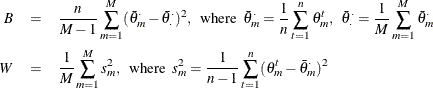
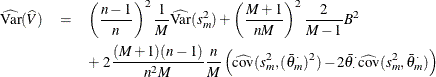
The posterior marginal variance, ![]() , is a weighted average of W and B. The estimate of the variance is
, is a weighted average of W and B. The estimate of the variance is
If all M chains have reached the target distribution, this posterior variance estimate should be very close to the within-chain variance
W. Therefore, you would expect to see the ratio ![]() be close to 1. The square root of this ratio is referred to as the potential scale reduction factor (PSRF). A large PSRF indicates that the between-chain variance is substantially greater than the within-chain variance, so
that longer simulation is needed. If the PSRF is close to 1, you can conclude that each of the M chains has stabilized, and they are likely to have reached the target distribution.
be close to 1. The square root of this ratio is referred to as the potential scale reduction factor (PSRF). A large PSRF indicates that the between-chain variance is substantially greater than the within-chain variance, so
that longer simulation is needed. If the PSRF is close to 1, you can conclude that each of the M chains has stabilized, and they are likely to have reached the target distribution.
A refined version of PSRF is calculated, as suggested by Brooks and Gelman (1997), as
where
and
All the Bayesian procedures also produce an upper ![]() confidence limit of
confidence limit of ![]() . Gelman and Rubin (1992) showed that the ratio
. Gelman and Rubin (1992) showed that the ratio ![]() in
in ![]() has an F distribution with degrees of freedom
has an F distribution with degrees of freedom ![]() and
and ![]() . Because you are concerned only if the scale is large, not small, only the upper
. Because you are concerned only if the scale is large, not small, only the upper ![]() confidence limit is reported. This is written as
confidence limit is reported. This is written as
![\[ \sqrt {\left( \frac{n-1}{n} + \frac{M+1}{nM} \cdot F_{1-\alpha /2} \left(M-1, \frac{2W^2}{\widehat{\mr {Var}}(s_ m^2)/M} \right) \right) \cdot \frac{\hat{d}+3}{\hat{d}+1}} \]](images/statug_introbayes0141.png)
In the Bayesian procedures, you can specify the number of chains that you want to run. Typically three chains are sufficient.
The first chain is used for posterior inference, such as mean and standard deviation; the other ![]() chains are used for computing the diagnostics and are discarded afterward. This test can be computationally costly, because
it prolongs the simulation M-fold.
chains are used for computing the diagnostics and are discarded afterward. This test can be computationally costly, because
it prolongs the simulation M-fold.
It is best to choose different initial values for all M chains. The initial values should be as dispersed from each other as possible so that the Markov chains can fully explore different parts of the distribution before they converge to the target. Similar initial values can be risky because all of the chains can get stuck in a local maximum; that is something this convergence test cannot detect. If you do not supply initial values for all the different chains, the procedures generate them for you.
The Geweke test (Geweke, 1992) compares values in the early part of the Markov chain to those in the latter part of the chain in order to detect failure
of convergence. The statistic is constructed as follows. Two subsequences of the Markov chain ![]() are taken out, with
are taken out, with ![]() and
and ![]() , where
, where ![]() . Let
. Let ![]() , and define
, and define
Let ![]() and
and ![]() denote consistent spectral density estimates at zero frequency (see the subsection Spectral Density Estimate at Zero Frequency for estimation details) for the two MCMC chains, respectively. If the ratios
denote consistent spectral density estimates at zero frequency (see the subsection Spectral Density Estimate at Zero Frequency for estimation details) for the two MCMC chains, respectively. If the ratios ![]() and
and ![]() are fixed,
are fixed, ![]() , and the chain is stationary, then the following statistic converges to a standard normal distribution as
, and the chain is stationary, then the following statistic converges to a standard normal distribution as ![]() :
:
![\[ Z_ n = \frac{\bar{\theta }_1 - \bar{\theta _2}}{\sqrt {\frac{\hat{s}_1(0)}{n_1} + \frac{\hat{s}_2(0)}{n_2}}} \]](images/statug_introbayes0153.png)
This is a two-sided test, and large absolute z-scores indicate rejection.
For one sequence of the Markov chain ![]() , the relationship between the h-lag covariance sequence of a time series and the spectral density, f, is
, the relationship between the h-lag covariance sequence of a time series and the spectral density, f, is
where i indicates that ![]() is the complex argument. Inverting this Fourier integral,
is the complex argument. Inverting this Fourier integral,
It follows that
which gives an autocorrelation adjusted estimate of the variance. In this equation, ![]() is the naive variance estimate of the sequence
is the naive variance estimate of the sequence ![]() and
and ![]() is the lag h autocorrelation. Due to obvious computational difficulties, such as calculation of autocorrelation at infinity, you cannot
effectively estimate
is the lag h autocorrelation. Due to obvious computational difficulties, such as calculation of autocorrelation at infinity, you cannot
effectively estimate ![]() by using the preceding formula. The usual route is to first obtain the periodogram
by using the preceding formula. The usual route is to first obtain the periodogram ![]() of the sequence, and then estimate
of the sequence, and then estimate ![]() by smoothing the estimated periodogram. The periodogram is defined to be
by smoothing the estimated periodogram. The periodogram is defined to be
![\[ p(\omega ) = \frac{1}{n} \left[ \left( \sum _{t=1}^{n} \theta _{t} \sin (\omega t) \right)^2 + \left( \sum _{t=1}^{n} \theta _{t} \cos (\omega t)\right)^2 \right] \]](images/statug_introbayes0164.png)
The procedures use the following way to estimate ![]() from p (Heidelberger and Welch, 1981). In
from p (Heidelberger and Welch, 1981). In ![]() , let
, let ![]() and
and ![]() .[3] A smooth spectral density in the domain of
.[3] A smooth spectral density in the domain of ![]() is obtained by fitting a gamma model with the log link function, using
is obtained by fitting a gamma model with the log link function, using ![]() as response and
as response and ![]() as the only regressor. The predicted value
as the only regressor. The predicted value ![]() is given by
is given by
where ![]() and
and ![]() are the estimates of the intercept and slope parameters, respectively.
are the estimates of the intercept and slope parameters, respectively.
The Heidelberger and Welch test (Heidelberger and Welch, 1981, 1983) consists of two parts: a stationary portion test and a half-width test. The stationarity test assesses the stationarity of a Markov chain by testing the hypothesis that the chain comes from a covariance stationary process. The half-width test checks whether the Markov chain sample size is adequate to estimate the mean values accurately.
Given ![]() , set
, set ![]() ,
, ![]() , and
, and ![]() . You can construct the following sequence with s coordinates on values from
. You can construct the following sequence with s coordinates on values from ![]() :
:
where ![]() is the rounding operator, and
is the rounding operator, and ![]() is an estimate of the spectral density at zero frequency that uses the second half of the sequence (see the section Spectral Density Estimate at Zero Frequency for estimation details). For large n,
is an estimate of the spectral density at zero frequency that uses the second half of the sequence (see the section Spectral Density Estimate at Zero Frequency for estimation details). For large n, ![]() converges in distribution to a Brownian bridge (Billingsley, 1986). So you can construct a test statistic by using
converges in distribution to a Brownian bridge (Billingsley, 1986). So you can construct a test statistic by using ![]() . The statistic used in these procedures is the Cramer–von Mises statistic[4]; that is
. The statistic used in these procedures is the Cramer–von Mises statistic[4]; that is ![]() . As
. As ![]() , the statistic converges in distribution to a standard Cramer–von Mises distribution. The integral
, the statistic converges in distribution to a standard Cramer–von Mises distribution. The integral ![]() is numerically approximated using Simpson’s rule.
is numerically approximated using Simpson’s rule.
Let ![]() , where
, where ![]() , and
, and ![]() . If n is even, let
. If n is even, let ![]() ; otherwise, let
; otherwise, let ![]() . The Simpson’s approximation to the integral is
. The Simpson’s approximation to the integral is
Note that Simpson’s rule requires an even number of intervals. When n is odd, ![]() is set to be 0 and the value does not contribute to the approximation.
is set to be 0 and the value does not contribute to the approximation.
This test can be performed repeatedly on the same chain, and it helps you identify a time t when the chain has reached stationarity. The whole chain, ![]() , is first used to construct the Cramer–von Mises statistic. If it passes the test, you can conclude that the entire chain
is stationary. If it fails the test, you drop the initial
, is first used to construct the Cramer–von Mises statistic. If it passes the test, you can conclude that the entire chain
is stationary. If it fails the test, you drop the initial ![]() of the chain and redo the test by using the remaining
of the chain and redo the test by using the remaining ![]() . This process is repeated until either a time t is selected or it reaches a point where there are not enough data remaining to construct a confidence interval (the cutoff
proportion is set to be
. This process is repeated until either a time t is selected or it reaches a point where there are not enough data remaining to construct a confidence interval (the cutoff
proportion is set to be ![]() ).
).
The part of the chain that is deemed stationary is put through a half-width test, which reports whether the sample size is
adequate to meet certain accuracy requirements for the mean estimates. Running the simulation less than this length of time
would not meet the requirement, while running it longer would not provide any additional information that is needed. The statistic
calculated here is the relative half-width (RHW) of the confidence interval. The RHW for a confidence interval of level ![]() is
is
where ![]() is the z-score of the
is the z-score of the ![]() percentile (for example,
percentile (for example, ![]() if
if ![]() ),
), ![]() is the variance of the chain estimated using the spectral density method (see explanation in the section Spectral Density Estimate at Zero Frequency), n is the length, and
is the variance of the chain estimated using the spectral density method (see explanation in the section Spectral Density Estimate at Zero Frequency), n is the length, and ![]() is the estimated mean. The RHW quantifies accuracy of the
is the estimated mean. The RHW quantifies accuracy of the ![]() level confidence interval of the mean estimate by measuring the ratio between the sample standard error of the mean and the
mean itself. In other words, you can stop the Markov chain if the variability of the mean stabilizes with respect to the mean.
An implicit assumption is that large means are often accompanied by large variances. If this assumption is not met, then this
test can produce false rejections (such as a small mean around 0 and large standard deviation) or false acceptance (such as
a very large mean with relative small variance). As with any other convergence diagnostics, you might want to exercise caution
in interpreting the results.
level confidence interval of the mean estimate by measuring the ratio between the sample standard error of the mean and the
mean itself. In other words, you can stop the Markov chain if the variability of the mean stabilizes with respect to the mean.
An implicit assumption is that large means are often accompanied by large variances. If this assumption is not met, then this
test can produce false rejections (such as a small mean around 0 and large standard deviation) or false acceptance (such as
a very large mean with relative small variance). As with any other convergence diagnostics, you might want to exercise caution
in interpreting the results.
The stationarity test is one-sided; rejection occurs when the p-value is greater than ![]() . To perform the half-width test, you need to select an
. To perform the half-width test, you need to select an ![]() level (the default of which is 0.05) and a predetermined tolerance value
level (the default of which is 0.05) and a predetermined tolerance value ![]() (the default of which is 0.1). If the calculated RHW is greater than
(the default of which is 0.1). If the calculated RHW is greater than ![]() , you conclude that there are not enough data to accurately estimate the mean with
, you conclude that there are not enough data to accurately estimate the mean with ![]() confidence under tolerance of
confidence under tolerance of ![]() .
.
If your interest lies in posterior percentiles, you want a diagnostic test that evaluates the accuracy of the estimated percentiles. The Raftery-Lewis test (Raftery and Lewis, 1992, 1995) is designed for this purpose. Notation and deductions here closely resemble those in Raftery and Lewis (1995).
Suppose you are interested in a quantity ![]() such that
such that ![]() , where q can be an arbitrary cumulative probability, such as 0.025. This
, where q can be an arbitrary cumulative probability, such as 0.025. This ![]() can be empirically estimated by finding the
can be empirically estimated by finding the ![]() th number of the sorted
th number of the sorted ![]() . Let
. Let ![]() denote the estimand, which corresponds to an estimated probability
denote the estimand, which corresponds to an estimated probability ![]() . Because the simulated posterior distribution converges to the true distribution as the simulation sample size grows,
. Because the simulated posterior distribution converges to the true distribution as the simulation sample size grows, ![]() can achieve any degree of accuracy if the simulator is run for a very long time. However, running too long a simulation can
be wasteful. Alternatively, you can use coverage probability to measure accuracy and stop the chain when a certain accuracy
is reached.
can achieve any degree of accuracy if the simulator is run for a very long time. However, running too long a simulation can
be wasteful. Alternatively, you can use coverage probability to measure accuracy and stop the chain when a certain accuracy
is reached.
A stopping criterion is reached when the estimated probability is within ![]() of the true cumulative probability q, with probability s, such as
of the true cumulative probability q, with probability s, such as ![]() . For example, suppose you want the coverage probability s to be 0.95 and the amount of tolerance r to be 0.005. This corresponds to requiring that the estimate of the cumulative distribution function of the 2.5th percentile
be estimated to within
. For example, suppose you want the coverage probability s to be 0.95 and the amount of tolerance r to be 0.005. This corresponds to requiring that the estimate of the cumulative distribution function of the 2.5th percentile
be estimated to within ![]() percentage points with probability 0.95.
percentage points with probability 0.95.
The Raftery-Lewis diagnostics test finds the number of iterations, M, that need to be discarded (burn-ins) and the number of iterations needed, N, to achieve a desired precision. Given a predefined cumulative probability q, these procedures first find ![]() , and then they construct a binary
, and then they construct a binary ![]() process
process ![]() by setting
by setting ![]() if
if ![]() and 0 otherwise for all t. The sequence
and 0 otherwise for all t. The sequence ![]() is itself not a Markov chain, but you can construct a subsequence of
is itself not a Markov chain, but you can construct a subsequence of ![]() that is approximately Markovian if it is sufficiently k-thinned. When k becomes reasonably large,
that is approximately Markovian if it is sufficiently k-thinned. When k becomes reasonably large, ![]() starts to behave like a Markov chain.
starts to behave like a Markov chain.
Next, the procedures find this thinning parameter k. The number k is estimated by comparing the Bayesian information criterion (BIC) between two Markov models: a first-order and a second-order
Markov model. A jth-order Markov model is one in which the current value of ![]() depends on the previous j values. For example, in a second-order Markov model,
depends on the previous j values. For example, in a second-order Markov model,
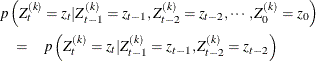
where ![]() . Given
. Given ![]() , you can construct two transition count matrices for a second-order Markov model:
, you can construct two transition count matrices for a second-order Markov model:
|
|
|
|||||
|
|
|
|
|
|||
|
|
|
|
|
|
|
|
|
|
|
|
|
|
|
|
For each k, the procedures calculate the BIC that compares the two Markov models. The BIC is based on a likelihood ratio test statistic that is defined as
where ![]() is the expected cell count of
is the expected cell count of ![]() under the null model, the first-order Markov model, where the assumption
under the null model, the first-order Markov model, where the assumption ![]() holds. The formula for the expected cell count is
holds. The formula for the expected cell count is
The BIC is ![]() , where
, where ![]() is the k-thinned sample size (every kth sample starting with the first), with the last two data points discarded due to the construction of the second-order Markov
model. The thinning parameter k is the smallest k for which the BIC is negative. When k is found, you can estimate a transition probability matrix between state 0 and state 1 for
is the k-thinned sample size (every kth sample starting with the first), with the last two data points discarded due to the construction of the second-order Markov
model. The thinning parameter k is the smallest k for which the BIC is negative. When k is found, you can estimate a transition probability matrix between state 0 and state 1 for ![]() :
:
Because ![]() is a Markov chain, its equilibrium distribution exists and is estimated by
is a Markov chain, its equilibrium distribution exists and is estimated by
where ![]() and
and ![]() . The goal is to find an iteration number m such that after m steps, the estimated transition probability
. The goal is to find an iteration number m such that after m steps, the estimated transition probability ![]() is within
is within ![]() of equilibrium
of equilibrium ![]() for
for ![]() . Let
. Let ![]() and
and ![]() . The estimated transition probability after step m is
. The estimated transition probability after step m is
which holds when
assuming ![]() .
.
Therefore, by time m, ![]() is sufficiently close to its equilibrium distribution, and you know that a total size of
is sufficiently close to its equilibrium distribution, and you know that a total size of ![]() should be discarded as the burn-in.
should be discarded as the burn-in.
Next, the procedures estimate N, the number of simulations needed to achieve desired accuracy on percentile estimation. The estimate of ![]() is
is ![]() . For large n,
. For large n, ![]() is normally distributed with mean q, the true cumulative probability, and variance
is normally distributed with mean q, the true cumulative probability, and variance
![]() is satisfied if
is satisfied if
Therefore, ![]() .
.
By using similar reasoning, the procedures first calculate the minimal number of iterations needed to achieve the desired accuracy, assuming the samples are independent:
If ![]() does not have that required sample size, the Raftery-Lewis test is not carried out. If you still want to carry out the test,
increase the number of Markov chain iterations.
does not have that required sample size, the Raftery-Lewis test is not carried out. If you still want to carry out the test,
increase the number of Markov chain iterations.
The ratio ![]() is sometimes referred to as the dependence factor. It measures deviation from posterior sample independence: the closer it is to 1, the less correlated are the samples. There
are a few things to keep in mind when you use this test. This diagnostic tool is specifically designed for the percentile
of interest and does not provide information about convergence of the chain as a whole (Brooks and Roberts, 1999). In addition, the test can be very sensitive to small changes. Both N and
is sometimes referred to as the dependence factor. It measures deviation from posterior sample independence: the closer it is to 1, the less correlated are the samples. There
are a few things to keep in mind when you use this test. This diagnostic tool is specifically designed for the percentile
of interest and does not provide information about convergence of the chain as a whole (Brooks and Roberts, 1999). In addition, the test can be very sensitive to small changes. Both N and ![]() are inversely proportional to
are inversely proportional to ![]() , so you can expect to see large variations in these numbers with small changes to input variables, such as the desired coverage
probability or the cumulative probability of interest. Last, the time until convergence for a parameter can differ substantially
for different cumulative probabilities.
, so you can expect to see large variations in these numbers with small changes to input variables, such as the desired coverage
probability or the cumulative probability of interest. Last, the time until convergence for a parameter can differ substantially
for different cumulative probabilities.
The sample autocorrelation of lag h for a parameter ![]() is defined in terms of the sample autocovariance function:
is defined in terms of the sample autocovariance function:
The sample autocovariance function of lag h of ![]() is defined by
is defined by
You can use autocorrelation and trace plots to examine the mixing of a Markov chain. A closely related measure of mixing is the effective sample size (ESS) (Kass et al., 1998).
where n is the total sample size and ![]() is the autocorrelation of lag k for
is the autocorrelation of lag k for ![]() . The quantity
. The quantity ![]() is referred to as the autocorrelation time. To estimate
is referred to as the autocorrelation time. To estimate ![]() , the Bayesian procedures first find a cutoff point k after which the autocorrelations are very close to zero, and then sum all the
, the Bayesian procedures first find a cutoff point k after which the autocorrelations are very close to zero, and then sum all the ![]() up to that point. The cutoff point k is such that
up to that point. The cutoff point k is such that ![]() , where
, where ![]() is the estimated standard deviation:
is the estimated standard deviation:
![\[ s_ k = \sqrt {\left( \frac{1}{n} \left( 1 + 2\sum _{j=1}^{k-1} \hat{\rho }_ j^2(\theta ) \right) \right)} \]](images/statug_introbayes0278.png)
ESS and ![]() are inversely proportional to each other, and low ESS or high
are inversely proportional to each other, and low ESS or high ![]() indicates bad mixing of the Markov chain.
indicates bad mixing of the Markov chain.