The VARIOGRAM Procedure

The following thick data set is available from the Sashelp library. The data set simulates measurements of coal seam thickness (in feet) taken over an approximately square area. The
Thick variable has the thickness values in the thick data set. The coordinates are offsets from a point in the southwest corner of the measurement area, with the north and east
distances in units of thousands of feet.
title 'Spatial Correlation Analysis with PROC VARIOGRAM';

data thick;
   input East North Thick @@;
   label Thick='Coal Seam Thickness';
   datalines;
 0.7  59.6  34.1   2.1  82.7  42.2   4.7  75.1  39.5
 4.8  52.8  34.3   5.9  67.1  37.0   6.0  35.7  35.9
 6.4  33.7  36.4   7.0  46.7  34.6   8.2  40.1  35.4
13.3   0.6  44.7  13.3  68.2  37.8  13.4  31.3  37.8
17.8   6.9  43.9  20.1  66.3  37.7  22.7  87.6  42.8
23.0  93.9  43.6  24.3  73.0  39.3  24.8  15.1  42.3
24.8  26.3  39.7  26.4  58.0  36.9  26.9  65.0  37.8
27.7  83.3  41.8  27.9  90.8  43.3  29.1  47.9  36.7
29.5  89.4  43.0  30.1   6.1  43.6  30.8  12.1  42.8
32.7  40.2  37.5  34.8   8.1  43.3  35.3  32.0  38.8
37.0  70.3  39.2  38.2  77.9  40.7  38.9  23.3  40.5
39.4  82.5  41.4  43.0   4.7  43.3  43.7   7.6  43.1
46.4  84.1  41.5  46.7  10.6  42.6  49.9  22.1  40.7
51.0  88.8  42.0  52.8  68.9  39.3  52.9  32.7  39.2
55.5  92.9  42.2  56.0   1.6  42.7  60.6  75.2  40.1
62.1  26.6  40.1  63.0  12.7  41.8  69.0  75.6  40.1
70.5  83.7  40.9  70.9  11.0  41.7  71.5  29.5  39.8
78.1  45.5  38.7  78.2   9.1  41.7  78.4  20.0  40.8
80.5  55.9  38.7  81.1  51.0  38.6  83.8   7.9  41.6
84.5  11.0  41.5  85.2  67.3  39.4  85.5  73.0  39.8
86.7  70.4  39.6  87.2  55.7  38.8  88.1   0.0  41.6
88.4  12.1  41.3  88.4  99.6  41.2  88.8  82.9  40.5
88.9   6.2  41.5  90.6   7.0  41.5  90.7  49.6  38.9
91.5  55.4  39.0  92.9  46.8  39.1  93.4  70.9  39.7
55.8  50.5  38.1  96.2  84.3  40.3  98.2  58.2  39.5
;
It is instructive to see the locations of the measured points in the area where you want to perform spatial prediction. It is desirable to have the sampling locations scattered evenly throughout the prediction area. If the locations are not scattered evenly, the prediction error might be unacceptably large where measurements are sparse.
You can run PROC VARIOGRAM in this preliminary analysis to determine potential problems. In the following statements, the NOVARIOGRAM option in the COMPUTE statement specifies that only the descriptive summaries and a plot of the raw data be produced.
ods graphics on;
proc variogram data=thick plots=pairs(thr=30);
   compute novariogram nhc=20;
   coordinates xc=East yc=North;
   var Thick;
run;
PROC VARIOGRAM produces the table in Figure 102.1 that shows the number of Thick observations read and used. This table provides you with useful information in case you have missing values in the input
data.
Figure 102.1: Number of Observations for the thick Data Set
| Spatial Correlation Analysis with PROC VARIOGRAM |
| Number of Observations Read | 75 |
|---|---|
| Number of Observations Used | 75 |
Then, the scatter plot of the observed data is produced as shown in Figure 102.2. According to the figure, although the locations are not ideally spread around the prediction area, there are not any extended areas lacking measurements. The same graph also provides the values of the measured variable by using colored markers.
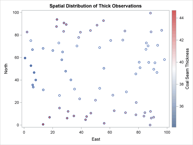
The following is a crucial step. Any obvious surface trend must be removed before you compute the empirical semivariogram and proceed to estimate a model of spatial dependence (the theoretical semivariogram model). You can observe in Figure 102.2 the small-scale variation typical of spatial data, but a first inspection indicates no obvious major systematic trend.
Assuming, therefore, that the data are free of surface trends, you can work with the original thickness rather than residuals obtained from a trend removal process. The following analysis also assumes that the spatial characterization is independent of the direction of the line that connects any two equidistant pairs of data; this is a property known as isotropy. See An Anisotropic Case Study with Surface Trend in the Data for a more detailed approach to trend analysis and the issue of anisotropy.
Following the previous exploratory analysis, you then need to classify each data pair as a member of a distance interval (lag). PROC VARIOGRAM performs this grouping with two required options for semivariogram computation: the LAGDISTANCE= and MAXLAGS= options. These options are based on your assessment of how to group the data pairs within distance classes.
The meaning of the required LAGDISTANCE= option is as follows. Classify all pairs of points into intervals according to their pairwise distance. The width of each distance interval is the LAGDISTANCE= value. The meaning of the required MAXLAGS= option is simply the number of intervals you consider. The problem is that given only the scatter plot of the measurement locations, it is not clear what values to give to the LAGDISTANCE= and MAXLAGS= options.
Ideally, you want a sufficient number of distance classes that capture the extent to which your data are correlated and you want each class to contain a minimum of data pairs to increase the accuracy in your computations. A rule of thumb used in semivariogram computations is that you should have at least 30 pairs per lag class. This is an empirical arbitrary threshold; see the section Choosing the Size of Classes for further details.
In the preliminary analysis, you use the option NHCLASSES= in the COMPUTE statement to help you experiment with these numbers and choose values for the LAGDISTANCE= and MAXLAGS= options. Here, in particular, you request NHCLASSES=20 to preview a classification that uses 20 distance classes across your spatial domain. A zero lag class is always considered; therefore the output shows the number of distance classes to be one more than the number you specified.
Based on your selection of the NHCLASSES= option, the NOVARIOGRAM option produces a pairwise distances table from your observations shown in Figure 102.3, and the corresponding histogram in Figure 102.4. For illustration purposes, you also specify a threshold of minimum data pairs per distance class in the PAIRS option as THR=30. As a result, a reference line appears in the histogram so that you can visually identify any lag classes with pairs that fall below your specified threshold.
Figure 102.3: Pairwise Distance Intervals Table
| Pairwise Distance Intervals | ||||
|---|---|---|---|---|
| Lag Class |
Bounds | Number of Pairs | Percentage of Pairs |
|
| 0 | 0.00 | 3.48 | 7 | 0.25% |
| 1 | 3.48 | 10.45 | 81 | 2.92% |
| 2 | 10.45 | 17.42 | 138 | 4.97% |
| 3 | 17.42 | 24.39 | 167 | 6.02% |
| 4 | 24.39 | 31.36 | 204 | 7.35% |
| 5 | 31.36 | 38.33 | 210 | 7.57% |
| 6 | 38.33 | 45.30 | 213 | 7.68% |
| 7 | 45.30 | 52.27 | 253 | 9.12% |
| 8 | 52.27 | 59.24 | 237 | 8.54% |
| 9 | 59.24 | 66.20 | 280 | 10.09% |
| 10 | 66.20 | 73.17 | 252 | 9.08% |
| 11 | 73.17 | 80.14 | 230 | 8.29% |
| 12 | 80.14 | 87.11 | 217 | 7.82% |
| 13 | 87.11 | 94.08 | 154 | 5.55% |
| 14 | 94.08 | 101.05 | 71 | 2.56% |
| 15 | 101.05 | 108.02 | 41 | 1.48% |
| 16 | 108.02 | 114.99 | 14 | 0.50% |
| 17 | 114.99 | 121.96 | 5 | 0.18% |
| 18 | 121.96 | 128.93 | 1 | 0.04% |
| 19 | 128.93 | 135.89 | 0 | 0.00% |
| 20 | 135.89 | 142.86 | 0 | 0.00% |
The NOVARIOGRAM option also produces a table with useful facts about the pairs and the distances between the most remote data in selected directions, shown in Figure 102.5. In particular, the lag distance value is calculated based on your selection of the NHCLASSES= option. The last three table entries report the overall maximum distance among your data pairs, in addition to the maximum distances in the main axes directions—that is, the vertical (N–S) axis and the horizontal (E–W) axis. This information is also provided in the inset of Figure 102.4. When you specify a threshold in the PAIRS suboption of the PLOTS option, as in this example, the threshold also appears in the table. Then, the line that follows indicates the highest lag class with the following property: each one of the distance classes that lie farther away from this lag features a pairs population below the specified threshold.
With the preceding information you can determine appropriate values for the LAGDISTANCE= and MAXLAGS= options in the COMPUTE statement. In particular, the classification that uses 20 distance classes is satisfactory, and you can choose LAGDISTANCE=7 after following the suggestion in Figure 102.5.
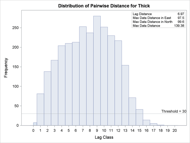
Figure 102.5: Pairs Information Table
| Pairs Information | |
|---|---|
| Number of Lags | 21 |
| Lag Distance | 6.97 |
| Minimum Pairs Threshold | 30 |
| Highest Lag With Pairs > Threshold | 15 |
| Maximum Data Distance in East | 97.50 |
| Maximum Data Distance in North | 99.60 |
| Maximum Data Distance | 139.38 |
The MAXLAGS= option needs to be specified based on the spatial extent to which your data are correlated. Unless you know this size, in the present omnidirectional case you can assume the correlation extent to be roughly equal to half the overall maximum distance between data points.
The table in Figure 102.5 suggests that this number corresponds to 139,380 feet, which is most likely on or close to a diagonal direction (that is,
the northeast–southwest or northwest–southeast direction). Hence, you can expect the correlation extent in this scale to be
around ![]() feet. Consequently, consider lag classes up to this distance for the empirical semivariogram computations. Given your lag
size selection, Figure 102.3 indicates that this distance corresponds to about 10 lags; hence you can set MAXLAGS=10.
feet. Consequently, consider lag classes up to this distance for the empirical semivariogram computations. Given your lag
size selection, Figure 102.3 indicates that this distance corresponds to about 10 lags; hence you can set MAXLAGS=10.
Overall, for a specific NHCLASSES= choice of class count, you can expect your choice of MAXLAGS= to be approximately half the number of the lag classes (see the section Spatial Extent of the Empirical Semivariogram for more details).
After you have starting values for the LAGDISTANCE= and MAXLAGS= options, you can run the VARIOGRAM procedure multiple times to inspect and compare the results you get by specifying different values for these options.