The QUANTLIFE Procedure (Experimental)

This example uses the human immunodeficiency virus (HIV) study data from Hosmer and Lemeshow (1999) to illustrate the basic features of PROC QUANTLIFE.
In this study, subjects were followed after a confirmed diagnosis of HIV. The primary goal was to evaluate the effect of various factors on the survival time. Two covariates for each subject were collected: age and history of prior intravenous drug use.
The following DATA step creates the data set HIV, which contains the variable Time (the follow-up time in days), the variable Status (with value 0 if Time was censored and 1 otherwise), the variable Drug (with value 1 for prior intravenous drug use and 0 otherwise), and the variable Age (the patient’s age in years at the beginning of the follow-up).
data HIV;
   input Time Age Drug Status;
   datalines;
    5      46      0        1
    6      35      1        0
    8      30      1        1
    3      30      1        1
   22      36      0        1
    1      32      1        0

   ... more lines ...

    1      34      1        1
 ;
You can use PROC QUANTLIFE to explore the relationship between the survival time and the two covariates at different quantiles.
Suppose you are interested in the median survivors and in the longer and shorter survivors. The following statements fit a linear model for the 25th, 50th, and 75th percentiles:
ods graphics on;
proc quantlife data=hiv log plots=quantplot seed=1268;
   class Drug;
   model Time*Status(0) = Drug Age / quantile=(0.25 0.5 0.75);
   Drug_Effect: test Drug;
run;
The LOG option fits a quantile regression model for the log of Time, as is done by an accelerated failure time (AFT) model in standard survival analysis. The SEED= option is specified to maintain
reproducibility of the resampling method that is used for statistical inference.
The MODEL statement specifies the response variable, Time, and the censoring variable, Censor. The value that indicates censoring is enclosed in parentheses. The values of Time are considered to be censored if the value of Censor is 0; otherwise, they are considered to be event times. The QUANTILE= option requests a fit of the conditional quantile function
![]() at the quantile levels 0.25, 0.5, and 0.75.
at the quantile levels 0.25, 0.5, and 0.75.
The TEST statement requests a test for the hypothesis that there is no Drug effect at each of the quantile levels.
Figure 76.1 displays basic model information. For example, you can see from Figure 76.1 that the response is log(Time), and the censoring rate is 20%.
Figure 76.1: Model Fitting Information
| Model Information | |
|---|---|
| Data Set | WORK.HIV |
| Dependent Variable | Log(Time) |
| Censoring Variable | Status |
| Censoring Value(s) | 0 |
| Number of Observations | 100 |
| Method | Kaplan-Meier |
| Replications | 200 |
| Seed for Random Number Generator | 1268 |
| Class Level Information | ||
|---|---|---|
| Name | Levels | Values |
| Drug | 2 | 0 1 |
| Summary of the Number of Event and Censored Values |
|||
|---|---|---|---|
| Total | Event | Censored | Percent Censored |
| 100 | 80 | 20 | 20.00 |
Figure 76.2 displays the parameter estimates, which are computed using the default Kaplan-Meier-type estimator. See the section Kaplan-Meier-Type Estimator for Censored Quantile Regression for details. In addition, Figure 76.2 displays standard errors, 95![]() confidence limits, t values, and p-values that are computed by the default resampling method, exponentially weighted resampling. See the section Exponentially Weighted Method.
confidence limits, t values, and p-values that are computed by the default resampling method, exponentially weighted resampling. See the section Exponentially Weighted Method.
A different quantile regression model is fitted for each quantile, and the first column (Quantile) in Figure 76.2 identifies the model for the parameter estimates. Age has a negative effect on survival time. You can use the parameter estimates to predict the survival time at the quantiles of interests. For example, the 75th percentile survival time for a person with no previous IV drug use at age 45 is
Figure 76.2: Parameter Estimates
| Parameter Estimates | |||||||||
|---|---|---|---|---|---|---|---|---|---|
| Quantile | Parameter | DF | Estimate | Standard Error |
95% Confidence Limits | t Value | Pr > |t| | ||
| 0.2500 | Intercept | 1 | 3.0373 | 1.1680 | 0.7482 | 5.3265 | 2.60 | 0.0108 | |
| Drug | 0 | 1 | 0.9516 | 0.4403 | 0.0887 | 1.8146 | 2.16 | 0.0331 | |
| Drug | 1 | 0 | 0 | 0 | 0 | 0 | . | . | |
| Age | 1 | -0.0646 | 0.0261 | -0.1158 | -0.0135 | -2.48 | 0.0150 | ||
| 0.5000 | Intercept | 1 | 5.3351 | 0.6605 | 4.0406 | 6.6296 | 8.08 | <.0001 | |
| Drug | 0 | 1 | 0.8681 | 0.2786 | 0.3219 | 1.4142 | 3.12 | 0.0024 | |
| Drug | 1 | 0 | 0 | 0 | 0 | 0 | . | . | |
| Age | 1 | -0.1059 | 0.0194 | -0.1439 | -0.0679 | -5.46 | <.0001 | ||
| 0.7500 | Intercept | 1 | 5.3351 | 0.9091 | 3.5532 | 7.1170 | 5.87 | <.0001 | |
| Drug | 0 | 1 | 1.1451 | 0.2625 | 0.6307 | 1.6596 | 4.36 | <.0001 | |
| Drug | 1 | 0 | 0 | 0 | 0 | 0 | . | . | |
| Age | 1 | -0.0941 | 0.0223 | -0.1378 | -0.0505 | -4.23 | <.0001 | ||
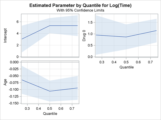
The PLOTS=QUANTPLOT option in the PROC QUANTLIFE statement requests the quantile process plots, which are shown in Figure 76.3. The quantile process plot is a scatter plot of an estimated regression. Figure 76.3 shows that the estimated coefficients for the two covariates does not change much across quantiles.
The tests that are requested by the TEST statement are shown in Figure 76.4.
Figure 76.4: Tests of Significance
| Test Drug_Effect Results | |||
|---|---|---|---|
| Quantile | DF | Chi-Square | Pr > ChiSq |
| 0.2500 | 1 | 4.67 | 0.0307 |
| 0.5000 | 1 | 9.70 | 0.0018 |
| 0.7500 | 1 | 19.03 | <.0001 |
The tests indicate that the coefficient of Drug is significantly different from 0 at the 25th, 50th, and 75th percentiles.