The QUANTLIFE Procedure (Experimental)

This example reproduces analysis done by Portnoy (2003), which demonstrates how to use quantile regression to analyze survival times. The example uses drug abuse data provided by Hosmer and Lemeshow (1999). The goal of this study is to compare treatment effects on reducing drug abuse.
The data set contains the following variables:
-
Time, time to return to drug use in days -
Status, event indicator with value 1 for return to drug use and value 0 for censored time -
Age, age in years at enrollment -
Treatment, with value 1 for six-month treatment and value 0 for three-month treatment -
Beck, Beck Depression Inventory score at admission to the program -
IV3, indicator of the recent IV drug use -
NDT, number of prior drug treatments. -
RACE, race indicator with value 1 for white and value 0 for nonwhite -
SITE, treatment sites (A and B) -
LOT, length (days) of treatment.
The following statements create the data set:
data uis;
   input  ID Age Becktota Hercoc Ivhx Ndrugtx Race Treat Site Lot Time
   Censor;
   Iv3 = (Ivhx = 3);
   Nd1 = 1/((Ndrugtx+1)/10);
   Nd2 = (1/((Ndrugtx+1)/10))*log((Ndrugtx+1)/10);
   if (Treat =1 ) then Frac = Lot/180;
   else  Frac = Lot/90;
   datalines;
     1  39   9.0000    4     3      1     0    1     0  123  188    1
     2  33  34.0000    4     2      8     0    1     0   25   26    1
     3  33  10.0000    2     3      3     0    1     0    7  207    1
     4  32  20.0000    4     3      1     0    0     0   66  144    1

   ... more lines ...

   626  28   10.0      4     2      3     0    1     1   21   35    1
   627  35   17.0      1     3      2     0    0     1  184  379    1
   628  46   31.5      1     3     15     1    1     1    9  377    1
;
The following statements replicate the analysis of Portnoy (2003):
ods graphics on;
proc quantlife data=uis log seed=999 plots=(quantplot survival);
   class Race Site Treat;
   model Time*Censor(0)=Nd1  Nd2  Iv3 Becktota
                        Treat  Frac  Race  Age|Site
                      / quantile=0.05 to 0.85 by 0.05 ;
   baseline out=Predsurvf survival=survf quantile=Time;

run;
Output 76.2.1 displays the model information. Out of 628 subjects, 53 contain missing values and are not included in the analysis. The censoring rate is 20.87%.
Output 76.2.1: Model Information
| Model Information | |
|---|---|
| Data Set | WORK.UIS |
| Dependent Variable | Log(Time) |
| Censoring Variable | Censor |
| Censoring Value(s) | 0 |
| Number of Observations | 575 |
| Method | Kaplan-Meier |
| Replications | 200 |
| Seed for Random Number Generator | 999 |
| Class Level Information | ||
|---|---|---|
| Name | Levels | Values |
| Race | 2 | 0 1 |
| Site | 2 | 0 1 |
| Treat | 2 | 0 1 |
| Summary of the Number of Event and Censored Values |
|||
|---|---|---|---|
| Total | Event | Censored | Percent Censored |
| 575 | 464 | 111 | 19.30 |
Output 76.2.2, Output 76.2.3, and Output 76.2.4 display regression quantile process plots for each covariate.
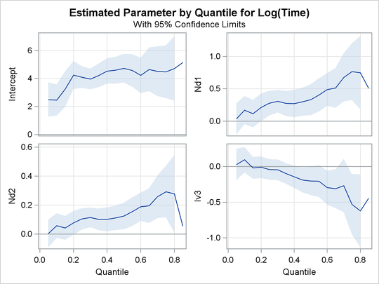
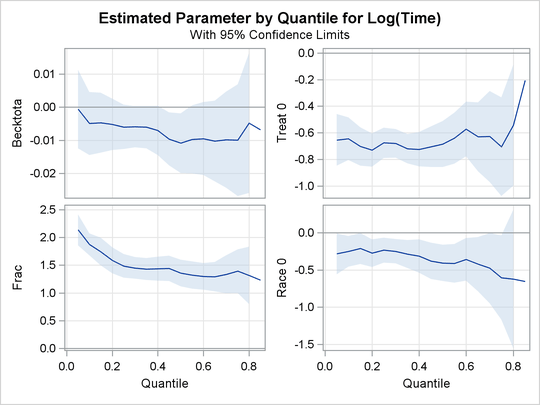
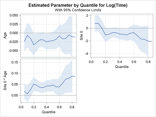
You can see the varying effects for Nd and Frac, while the treatment effect is fairly constant. See Portnoy (2003) for more details about the covariate effects that can be discovered with quantile regression.
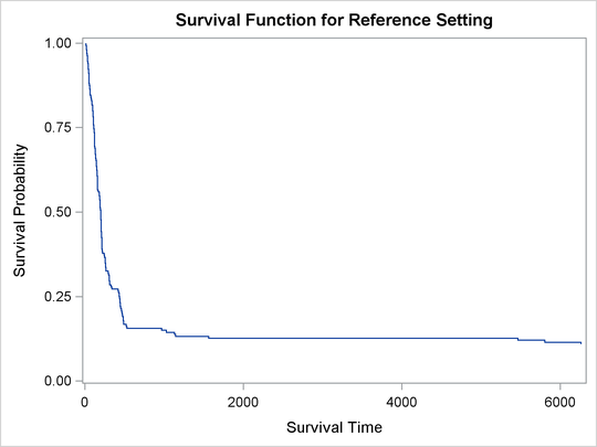
In survival analysis, a plot of the estimated survival function is often of interest. There is a one-to-one relationship between the quantile function and the survival function. When you specify the PLOTS= SURVIVAL option, the QUANTLIFE procedure estimates the survival function by fitting a quantile regression model for a grid of equally spaced quantile levels. You can specify the grid points with the INITTAU=option and the step between adjacent grid points with the GRIDSIZE=option. See the section Kaplan-Meier-Type Estimator for Censored Quantile Regression for more information.
Figure 76.4 shows the estimated survival function at the reference set of covariate values that consist of reference levels for the CLASS variables and average values for the continuous variables. You can output the predicted survival function by specifying the SURVIVAL= option in the BASELINE statement.