The QUANTLIFE Procedure (Experimental)

This example illustrates how to detect varying covariate effects on survival time with quantile regression analysis. Consider a study of primary biliary cirrhosis, a rare but fatal chronic liver disease discussed by Fleming and Harrington (1991). Researchers followed 418 patients with this disease, of whom 161 died during the study.
The data set contains the following variables:
-
Time, follow-up time, in years -
Status, event indicator with value 1 for death time and value 0 for censored time -
Age, age in years from birth to study registration -
Albumin, serum albumin level, in gm/dl -
Bilirubin, serum bilirubin level, in mg/dl -
Edema, edema presence -
Protime, prothrombin time, in seconds
The following statements create the data set PBC that is used in this example:
data pbc;
   input Time Status Age Albumin Bilirubin Edema Protime @@;
   label Time="Follow-up Time in Days";
   logAlbumin   = log(Albumin);
   logBilirubin = log(Bilirubin);
   logProtime   = log(Protime);
   datalines;
  400 1 58.7652 2.60 14.5 1.0 12.2 4500 0 56.4463 4.14  1.1 0.0 10.6
 1012 1 70.0726 3.48  1.4 0.5 12.0 1925 1 54.7406 2.54  1.8 0.5 10.3
 1504 0 38.1054 3.53  3.4 0.0 10.9 2503 1 66.2587 3.98  0.8 0.0 11.0
 1832 0 55.5346 4.09  1.0 0.0  9.7 2466 1 53.0568 4.00  0.3 0.0 11.0
 2400 1 42.5079 3.08  3.2 0.0 11.0   51 1 70.5599 2.74 12.6 1.0 11.5
 3762 1 53.7139 4.16  1.4 0.0 12.0  304 1 59.1376 3.52  3.6 0.0 13.6

   ... more lines ...

  989 0 35.0000 3.23  0.7 0.0 10.8  681 1 67.0000 2.96  1.2 0.0 10.9
 1103 0 39.0000 3.83  0.9 0.0 11.2 1055 0 57.0000 3.42  1.6 0.0  9.9
  691 0 58.0000 3.75  0.8 0.0 10.4  976 0 53.0000 3.29  0.7 0.0 10.6
;
The next statements fit a linear model for the log of survival time of the PBC patients with the covariates logBilirubin, logProtime, logAlbumin, Age, and Edema.
ods graphics on;
proc quantlife data=pbc log method=na plot=(quantplot survival) seed=1268;
   model Time*Status(0)=logBilirubin logProtime logAlbumin Age Edema
                        /quantile=(.1 .2 .3 .4 .5 .6 .75);
run;
You use the QUANTILE= option to specify a set of quantiles of interest for comparing quantile-specific covariate effects. The METHOD= option specifies the Nelson-Aalen method for estimating the regression parameters.
The QUANTLIFE procedure provides resampling methods for computing confidence limits for the parameters; see the section Confidence Interval for details. By default, the repetition number is 200. You can request a different number of repetitions with the NREP= option. You can also use the SEED= option to specify the seed for generating random numbers so that you can later reproduce the results.
Output 76.1.1 displays model information and information about censoring in the data. Out of 418 observations, 257 are censored.
Output 76.1.1: Model Information
| Model Information | |
|---|---|
| Data Set | WORK.PBC |
| Dependent Variable | Log(Time) |
| Censoring Variable | Status |
| Censoring Value(s) | 0 |
| Number of Observations | 418 |
| Method | Nelson-Aalen |
| Replications | 200 |
| Seed for Random Number Generator | 1268 |
| Summary of the Number of Event and Censored Values |
|||
|---|---|---|---|
| Total | Event | Censored | Percent Censored |
| 418 | 161 | 257 | 61.48 |
Output 76.1.2 provides the parameter estimates. Each quantile level has a set of parameter estimates and confidence limits.
Output 76.1.2: Parameter Estimates at Different Quantiles
| Parameter Estimates | ||||||||
|---|---|---|---|---|---|---|---|---|
| Quantile | Parameter | DF | Estimate | Standard Error |
95% Confidence Limits | t Value | Pr > |t| | |
| 0.1000 | Intercept | 1 | 14.8030 | 4.0967 | 6.7736 | 22.8325 | 3.61 | 0.0003 |
| logBilirubin | 1 | -0.4488 | 0.1485 | -0.7398 | -0.1578 | -3.02 | 0.0027 | |
| logProtime | 1 | -3.6378 | 1.4560 | -6.4915 | -0.7841 | -2.50 | 0.0129 | |
| logAlbumin | 1 | 1.9286 | 0.9756 | 0.0165 | 3.8408 | 1.98 | 0.0487 | |
| Age | 1 | -0.0244 | 0.0107 | -0.0455 | -0.00334 | -2.27 | 0.0237 | |
| Edema | 1 | -1.0712 | 0.6688 | -2.3820 | 0.2396 | -1.60 | 0.1100 | |
| 0.2000 | Intercept | 1 | 15.1800 | 2.6664 | 9.9540 | 20.4060 | 5.69 | <.0001 |
| logBilirubin | 1 | -0.6532 | 0.0886 | -0.8268 | -0.4796 | -7.37 | <.0001 | |
| logProtime | 1 | -3.3273 | 0.9401 | -5.1699 | -1.4847 | -3.54 | 0.0004 | |
| logAlbumin | 1 | 1.6842 | 0.6888 | 0.3343 | 3.0342 | 2.45 | 0.0149 | |
| Age | 1 | -0.0291 | 0.00687 | -0.0425 | -0.0156 | -4.23 | <.0001 | |
| Edema | 1 | -0.7265 | 0.3179 | -1.3497 | -0.1034 | -2.29 | 0.0228 | |
| 0.3000 | Intercept | 1 | 13.2382 | 2.5296 | 8.2804 | 18.1961 | 5.23 | <.0001 |
| logBilirubin | 1 | -0.6013 | 0.0762 | -0.7506 | -0.4521 | -7.90 | <.0001 | |
| logProtime | 1 | -2.5816 | 0.8907 | -4.3273 | -0.8359 | -2.90 | 0.0039 | |
| logAlbumin | 1 | 1.7246 | 0.7142 | 0.3248 | 3.1245 | 2.41 | 0.0162 | |
| Age | 1 | -0.0244 | 0.00716 | -0.0385 | -0.0104 | -3.41 | 0.0007 | |
| Edema | 1 | -0.8577 | 0.2763 | -1.3992 | -0.3163 | -3.10 | 0.0020 | |
| 0.4000 | Intercept | 1 | 13.4716 | 3.0874 | 7.4204 | 19.5228 | 4.36 | <.0001 |
| logBilirubin | 1 | -0.6047 | 0.0846 | -0.7705 | -0.4389 | -7.15 | <.0001 | |
| logProtime | 1 | -2.1632 | 1.1726 | -4.4615 | 0.1351 | -1.84 | 0.0658 | |
| logAlbumin | 1 | 0.9819 | 0.7191 | -0.4274 | 2.3912 | 1.37 | 0.1728 | |
| Age | 1 | -0.0255 | 0.00681 | -0.0389 | -0.0122 | -3.74 | 0.0002 | |
| Edema | 1 | -1.0589 | 0.3104 | -1.6672 | -0.4506 | -3.41 | 0.0007 | |
| 0.5000 | Intercept | 1 | 10.9205 | 2.8047 | 5.4235 | 16.4175 | 3.89 | 0.0001 |
| logBilirubin | 1 | -0.5315 | 0.0904 | -0.7087 | -0.3543 | -5.88 | <.0001 | |
| logProtime | 1 | -1.2222 | 1.2142 | -3.6020 | 1.1577 | -1.01 | 0.3148 | |
| logAlbumin | 1 | 1.5700 | 0.6284 | 0.3383 | 2.8016 | 2.50 | 0.0129 | |
| Age | 1 | -0.0318 | 0.00883 | -0.0491 | -0.0145 | -3.60 | 0.0004 | |
| Edema | 1 | -0.7316 | 0.3743 | -1.4653 | 0.00202 | -1.95 | 0.0513 | |
| 0.6000 | Intercept | 1 | 11.2381 | 2.6294 | 6.0846 | 16.3917 | 4.27 | <.0001 |
| logBilirubin | 1 | -0.5701 | 0.0852 | -0.7370 | -0.4031 | -6.69 | <.0001 | |
| logProtime | 1 | -1.3508 | 1.1402 | -3.5856 | 0.8840 | -1.18 | 0.2368 | |
| logAlbumin | 1 | 1.3704 | 0.5091 | 0.3726 | 2.3682 | 2.69 | 0.0074 | |
| Age | 1 | -0.0226 | 0.0109 | -0.0440 | -0.00111 | -2.06 | 0.0399 | |
| Edema | 1 | -0.5141 | 0.3088 | -1.1193 | 0.0912 | -1.66 | 0.0968 | |
| 0.7500 | Intercept | 1 | 10.0954 | 3.1893 | 3.8445 | 16.3463 | 3.17 | 0.0017 |
| logBilirubin | 1 | -0.6366 | 0.1071 | -0.8466 | -0.4267 | -5.94 | <.0001 | |
| logProtime | 1 | -0.9670 | 1.2343 | -3.3862 | 1.4521 | -0.78 | 0.4338 | |
| logAlbumin | 1 | 1.8148 | 0.5883 | 0.6618 | 2.9678 | 3.08 | 0.0022 | |
| Age | 1 | -0.0203 | 0.0156 | -0.0509 | 0.0102 | -1.30 | 0.1931 | |
| Edema | 1 | -0.3529 | 0.3120 | -0.9644 | 0.2586 | -1.13 | 0.2587 | |
For comparison, the following statements use the LIFEREG procedure to fit a Weibull distribution to the data. The LIFEREG procedure fits an accelerated failure time model, which assumes that the effect of independent variables is multiplicative on the event time.
proc lifereg data=pbc;
   model Time*Status(0)=logBilirubin logProtime logAlbumin Age Edema;
run;
Output 76.1.3 provides the parameter estimates that are computed by PROC LIFEREG.
Output 76.1.3: Parameter Estimates From PROC LIFEREG
| Analysis of Maximum Likelihood Parameter Estimates | |||||||
|---|---|---|---|---|---|---|---|
| Parameter | DF | Estimate | Standard Error | 95% Confidence Limits | Chi-Square | Pr > ChiSq | |
| Intercept | 1 | 12.2155 | 1.4539 | 9.3658 | 15.0651 | 70.59 | <.0001 |
| logBilirubin | 1 | -0.5770 | 0.0556 | -0.6861 | -0.4680 | 107.55 | <.0001 |
| logProtime | 1 | -1.7565 | 0.5248 | -2.7850 | -0.7280 | 11.20 | 0.0008 |
| logAlbumin | 1 | 1.6694 | 0.4276 | 0.8313 | 2.5074 | 15.24 | <.0001 |
| Age | 1 | -0.0265 | 0.0053 | -0.0368 | -0.0162 | 25.35 | <.0001 |
| Edema | 1 | -0.6303 | 0.1805 | -0.9842 | -0.2764 | 12.19 | 0.0005 |
| Scale | 1 | 0.6807 | 0.0430 | 0.6014 | 0.7704 | ||
| Weibull Shape | 1 | 1.4691 | 0.0928 | 1.2980 | 1.6628 | ||
The p-value for logProtime is very small. For this same variable, the p-values that result from the quantile regression analysis are 0.3148 for the 0.5th quantile and 0.4338 for the 0.75th quantile,
and the p-values are much smaller for the lower quantiles. Apparently, the effect of this covariate depends on which side of the response
distribution is being modeled.
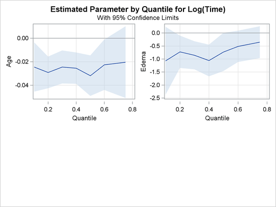
The PLOT=QUANTPLOT option in the PROC QUANTLIFE statement requests the quantile process plots in Output 76.1.4 and Output 76.1.5. These displays plot the estimated regression parameter against the quantile level. You can use these plots to compare quantile-specific
covariate effects. If the curve is not constant, it can indicate heterogeneity in the data. The interpretation of the regression
coefficients at a given quantile is similar to classical regression analysis. That is, the coefficient from a given covariate
indicates the effect on log(Time) of a unit change in that covariate, assuming that the other covariates are fixed.
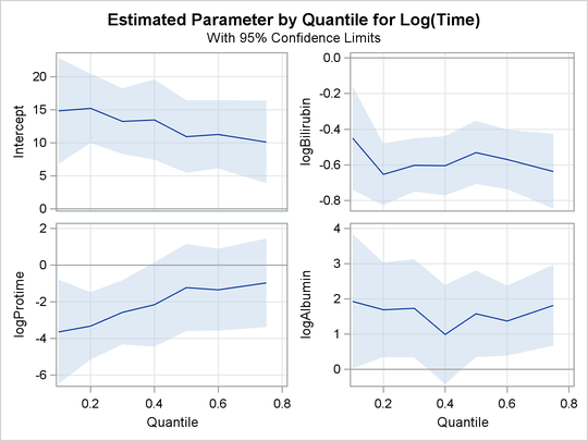
In the first panel, you can see that the effect of logProtime has a negative effect over the lower quantiles, which diminishes in magnitude at the median and upper quantiles. This insight
would be missed with the accelerated failure model.