The SEQTEST Procedure
- Overview
- Getting Started
-
Syntax

-
Details
Input Data Sets Boundary Variables Information Level Adjustments at Future Stages Boundary Adjustments for Information Levels Boundary Adjustments for Minimum Error Spending Boundary Adjustments for Overlapping Lower and Upper beta Boundaries Stochastic Curtailment Repeated Confidence Intervals Analysis after a Sequential Test Available Sample Space Orderings in a Sequential Test Applicable Tests and Sample Size Computation Table Output ODS Table Names Graphics Output ODS Graphics Acknowledgments
-
Examples
Testing the Difference between Two Proportions Testing an Effect in a Regression Model Testing an Effect with Early Stopping to Accept H0 Testing a Binomial Proportion Comparing Two Proportions with a Log Odds Ratio Test Comparing Two Survival Distributions with a Log-Rank Test Testing an Effect in a Proportional Hazards Regression Model Testing an Effect in a Logistic Regression Model
- References
Example 81.5 Comparing Two Proportions with a Log Odds Ratio Test
This example compares two binomial proportions by using a log odds ratio statistic in a five-stage group sequential test. A clinic is studying the effect of vitamin C supplements in treating flu symptoms. The study consists of patients in the clinic who exhibit the first sign of flu symptoms within the last 24 hours. These patients are randomly assigned to either the control group (which receives placebo pills) or the treatment group (which receives large doses of vitamin C supplements). At the end of a five-day period, the flu symptoms of each patient are recorded.
Suppose that you know from past experience that flu symptoms disappear in five days for  of patients who experience flu symptoms. The clinic would like to detect a
  symptom disappearance with a high probability. A test that compares the proportions directly specifies the null hypothesis
 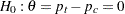 with a one-sided alternative
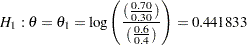
  and a power of
  at
at  , where
  and
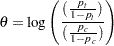
and  are the proportions of symptom disappearance in the treatment group and control group, respectively. An alternative trial tests an equivalent hypothesis by using the log odds ratio statistics:
 |
Then the null hypothesis is  and the alternative hypothesis is
 |
The following statements invoke the SEQDESIGN procedure and request a five-stage group sequential design by using an error spending function method for normally distributed statistics. The design uses a two-sided alternative hypothesis with early stopping to reject the null hypothesis  .
.
ods graphics on;
proc seqdesign altref=0.441833
               boundaryscale=mle
               ;
   OneSidedErrorSpending: design method=errfuncpow
                                 nstages=5
                                 alt=upper
                                 stop=accept
                                 alpha=0.025;
   samplesize model=twosamplefreq( nullprop=0.6 test=logor);
ods output Boundary=Bnd_CSup;
run;
ods graphics off;
The ODS OUTPUT statement with the BOUNDARY=BND_CSUP option creates an output data set named BND_CSUP which contains the resulting boundary information for the subsequent sequential tests.
The "Design Information" table in Output 81.5.1 displays design specifications and derived statistics. With the specified alternative reference, the maximum information  is derived.
| Design Information | |
|---|---|
| Statistic Distribution | Normal |
| Boundary Scale | MLE |
| Alternative Hypothesis | Upper |
| Early Stop | Accept Null |
| Method | Error Spending |
| Boundary Key | Both |
| Alternative Reference | 0.441833 |
| Number of Stages | 5 |
| Alpha | 0.025 |
| Beta | 0.1 |
| Power | 0.9 |
| Max Information (Percent of Fixed Sample) | 104.6166 |
| Max Information | 56.30934 |
| Null Ref ASN (Percent of Fixed Sample) | 57.21399 |
| Alt Ref ASN (Percent of Fixed Sample) | 102.1058 |
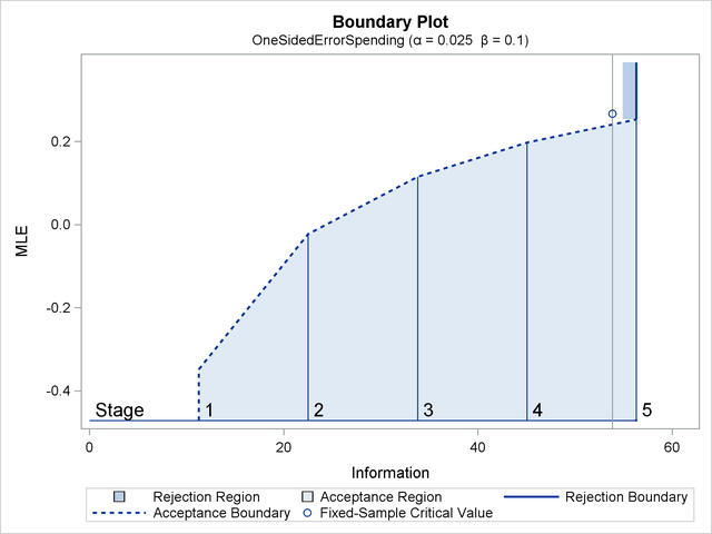
The "Boundary Information" table in Output 81.5.2 displays information level, alternative reference, and boundary values at each stage. With the specified BOUNDARYSCALE=MLE option, the procedure displays the output boundaries in terms of the MLE scale.
| Boundary Information (MLE Scale) Null Reference = 0 |
|||||
|---|---|---|---|---|---|
| _Stage_ | Alternative | Boundary Values | |||
| Information Level | Reference | Upper | |||
| Proportion | Actual | N | Upper | Beta | |
| 1 | 0.2000 | 11.26187 | 201.1048 | 0.44183 | -0.34844 |
| 2 | 0.4000 | 22.52374 | 402.2096 | 0.44183 | -0.02262 |
| 3 | 0.6000 | 33.7856 | 603.3144 | 0.44183 | 0.11527 |
| 4 | 0.8000 | 45.04747 | 804.4192 | 0.44183 | 0.19708 |
| 5 | 1.0000 | 56.30934 | 1005.524 | 0.44183 | 0.25345 |
With ODS Graphics enabled, a detailed boundary plot with the rejection and acceptance regions is displayed, as shown in Output 81.5.3.
With the SAMPLESIZE statement, the "Sample Size Summary" table in Output 81.5.4 displays the parameters for the sample size computation.
| Sample Size Summary | |
|---|---|
| Test | Two-Sample Proportions |
| Null Proportion | 0.6 |
| Proportion (Group A) | 0.7 |
| Test Statistic | Log Odds Ratio |
| Reference Proportions | Alt Ref |
| Max Sample Size | 1005.524 |
| Expected Sample Size (Null Ref) | 549.9132 |
| Expected Sample Size (Alt Ref) | 981.3914 |
The "Sample Sizes" table in Output 81.5.5 displays the required sample sizes for the group sequential clinical trial.
| Sample Sizes (N) Two-Sample Log Odds Ratio Test for Proportion Difference |
||||||||
|---|---|---|---|---|---|---|---|---|
| _Stage_ | Fractional N | Ceiling N | ||||||
| N | N(Grp 1) | N(Grp 2) | Information | N | N(Grp 1) | N(Grp 2) | Information | |
| 1 | 201.10 | 100.55 | 100.55 | 11.2619 | 202 | 101 | 101 | 11.3120 |
| 2 | 402.21 | 201.10 | 201.10 | 22.5237 | 404 | 202 | 202 | 22.6240 |
| 3 | 603.31 | 301.66 | 301.66 | 33.7856 | 604 | 302 | 302 | 33.8240 |
| 4 | 804.42 | 402.21 | 402.21 | 45.0475 | 806 | 403 | 403 | 45.1360 |
| 5 | 1005.52 | 502.76 | 502.76 | 56.3093 | 1006 | 503 | 503 | 56.3360 |
Thus,  new patients are needed in each group at stages
  ,
,  , and
, and  , and
, and  new patients are needed in each group at stages
  and
and  . Suppose that patients are available in each group at stage . Output 81.5.6 lists the
  observations in the data set count_1.
| First 10 Obs in the Trial Data |
| Obs | TrtGrp | Resp |
|---|---|---|
| 1 | Control | 1 |
| 2 | C_Sup | 0 |
| 3 | Control | 0 |
| 4 | C_Sup | 1 |
| 5 | Control | 1 |
| 6 | C_Sup | 1 |
| 7 | Control | 1 |
| 8 | C_Sup | 0 |
| 9 | Control | 0 |
| 10 | C_Sup | 1 |
The TrtGrp variable is a grouping variable with the value Control for a patient in the placebo control group and the value C_Sup for a patient in the treatment group who receives vitamin C supplements. The Resp variable is an indicator variable with the value for a patient without flu symptoms after five days and the value  for a patient with flu symptoms after five days.
The following statements use the LOGISTIC procedure to compute the log odds ratio statistic and its associated standard error at stage :
proc logistic data=CSup_1 descending;
   class TrtGrp / param=ref;
   model Resp= TrtGrp;
   ods output ParameterEstimates=Parms_CSup1;
run;
The DESCENDING option is used to reverse the order for the response levels, so the LOGISTIC procedure is modeling the probability that Resp = .
The following statements create and display (in Output 81.5.7) the data set for the log odds ratio statistic and its associated standard error:
data Parms_CSup1;
   set Parms_CSup1;
   if Variable='TrtGrp' and ClassVal0='C_Sup';
   _Scale_='MLE';
   _Stage_= 1;
   keep _Scale_ _Stage_ Variable Estimate StdErr;
run;

proc print data=Parms_CSup1;
   title 'Statistics Computed at Stage 1';
run;
| Statistics Computed at Stage 1 |
| Obs | Variable | Estimate | StdErr | _Scale_ | _Stage_ |
|---|---|---|---|---|---|
| 1 | TrtGrp | 0.3247 | 0.2856 | MLE | 1 |
The following statements invoke the SEQTEST procedure to test for early stopping at stage :
ods graphics on;
proc seqtest Boundary=Bnd_CSup
             Parms(Testvar=TrtGrp)=Parms_CSup1
             infoadj=prop
             errspendadj=errfuncpow
             boundarykey=both
             boundaryscale=mle
             ;
ods output test=Test_CSup1; run;
ods graphics off;
The BOUNDARY= option specifies the input data set that provides the boundary information for the trial at stage , which was generated in the SEQDESIGN procedure. The PARMS=PARMS_CSUP1 option specifies the input data set PARMS_CSUP1 that contains the test statistic and its associated standard error at stage , and the TESTVAR=TRTGRP option identifies the test variable TRTGRP in the data set.
If the computed information level for stage is not the same as the value provided in the BOUNDARY= data set, the INFOADJ=PROP option (which is the default) proportionally adjusts the information levels at future interim stages from the levels provided in the BOUNDARY= data set. The ERRSPENDADJ=ERRFUNCPOW option adjusts the boundaries with the updated error spending values generated from the power error spending function. The BOUNDARYKEY=BOTH option maintains both the  and
and  levels. The BOUNDARYSCALE=MLE option displays the output boundaries in terms of the MLE scale.
The ODS OUTPUT statement with the TEST=TEST_CSUP1 option creates an output data set named TEST_CSUP1 which contains the updated boundary information for the test at stage . The data set also provides the boundary information that is needed for the group sequential test at the next stage.
The "Design Information" table in Output 81.5.8 displays design specifications. With the specified BOUNDARYKEY=BOTH option, the information levels and boundary values at future stages are modified to maintain both the and levels.
| Design Information | |
|---|---|
| BOUNDARY Data Set | WORK.BND_CSUP |
| Data Set | WORK.PARMS_CSUP1 |
| Statistic Distribution | Normal |
| Boundary Scale | MLE |
| Alternative Hypothesis | Upper |
| Early Stop | Accept Null |
| Number of Stages | 5 |
| Alpha | 0.025 |
| Beta | 0.1 |
| Power | 0.9 |
| Max Information (Percent of Fixed Sample) | 104.6673 |
| Max Information | 56.3361718 |
| Null Ref ASN (Percent of Fixed Sample) | 57.02894 |
| Alt Ref ASN (Percent of Fixed Sample) | 102.1369 |
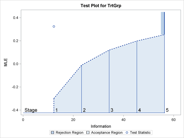
The "Test Information" table in Output 81.5.9 displays the boundary values for the test statistic with the specified MLE scale. With the INFOADJ=PROP option (which is the default), the information levels at future interim stages are derived proportionally from the observed information at stage and the information levels in the BOUNDARY= data set.
Since the information level at stage is derived from the PARMS= data set and other information levels are not specified, equal increments are used at remaining stages. At stage , the MLE statistic  is greater than the corresponding upper boundary value
  , so the sequential test continues to the next stage.
| Test Information (MLE Scale) Null Reference = 0 |
||||||
|---|---|---|---|---|---|---|
| _Stage_ | Alternative | Boundary Values | Test | |||
| Information Level | Reference | Upper | TrtGrp | |||
| Proportion | Actual | Upper | Beta | Estimate | Action | |
| 1 | 0.2176 | 12.26014 | 0.44183 | -0.29906 | 0.32474 | Continue |
| 2 | 0.4132 | 23.27914 | 0.44183 | -0.01067 | . | |
| 3 | 0.6088 | 34.29815 | 0.44183 | 0.11942 | . | |
| 4 | 0.8044 | 45.31716 | 0.44183 | 0.19829 | . | |
| 5 | 1.0000 | 56.33617 | 0.44183 | 0.25325 | . | |
With ODS Graphics enabled, a boundary plot with the boundary values and test statistics is displayed, as shown in Output 81.5.10. As expected, the test statistic is in the continuation region.
The following statements use the LOGISTIC procedure to compute the log odds ratio statistic and its associated standard error at stage :
proc logistic data=CSup_2 descending;
   class TrtGrp / param=ref;
   model Resp= TrtGrp;
   ods output ParameterEstimates=Parms_CSup2;
run;
The following statements create and display (in Output 81.5.11) the data set for the mean positive response and its associated standard error at stage :
data Parms_CSup2;
   set Parms_CSup2;
   if Variable='TrtGrp' and ClassVal0='C_Sup';
   _Scale_='MLE';
   _Stage_= 2;
   keep _Scale_ _Stage_ Variable Estimate StdErr;
run;
proc print data=Parms_CSup2;
   title 'Statistics Computed at Stage 2';
run;
| Statistics Computed at Stage 2 |
| Obs | Variable | Estimate | StdErr | _Scale_ | _Stage_ |
|---|---|---|---|---|---|
| 1 | TrtGrp | 0.2356 | 0.2073 | MLE | 2 |
The following statements invoke the SEQTEST procedure to test for early stopping at stage :
proc seqtest Boundary=Test_CSup1
             Parms( testvar=TrtGrp)=Parms_CSup2
             infoadj=prop
             errspendadj=errfuncpow
             boundarykey=both
             boundaryscale=mle
             ;
ods output Test=Test_CSup2;
run;
The BOUNDARY= option specifies the input data set that provides the boundary information for the trial at stage , which was generated by the SEQTEST procedure at the previous stage. The PARMS= option specifies the input data set that contains the test statistic and its associated standard error at stage , and the TESTVAR= option identifies the test variable in the data set.
The ODS OUTPUT statement with the TEST=CSUP_LDL2 option creates an output data set named CSUP_LDL2 which contains the updated boundary information for the test at stage . The data set also provides the boundary information that is needed for the group sequential test at the next stage.
The "Test Information" table in Output 81.5.12 displays the boundary values for the test statistic with the specified MLE scale. The test statistic  is greater than the corresponding upper boundary value
  , so the sequential test continues to the next stage.
| Test Information (MLE Scale) Null Reference = 0 |
||||||
|---|---|---|---|---|---|---|
| _Stage_ | Alternative | Boundary Values | Test | |||
| Information Level | Reference | Upper | TrtGrp | |||
| Proportion | Actual | Upper | Beta | Estimate | Action | |
| 1 | 0.2176 | 12.26014 | 0.44183 | -0.29906 | 0.32474 | Continue |
| 2 | 0.4132 | 23.27916 | 0.44183 | -0.01068 | 0.23560 | Continue |
| 3 | 0.6088 | 34.29799 | 0.44183 | 0.11942 | . | |
| 4 | 0.8044 | 45.31681 | 0.44183 | 0.19829 | . | |
| 5 | 1.0000 | 56.33563 | 0.44183 | 0.25325 | . | |
Similar results are found at stages and stage , so the trial continues to the final stage. The following statements use the LOGISTIC procedure to compute the log odds ratio statistic and its associated standard error at stage :
proc logistic data=CSup_5 descending;
   class TrtGrp / param=ref;
   model Resp= TrtGrp;
   ods output ParameterEstimates=Parms_CSup5;
run;
The following statements create and display (in Output 81.5.13) the data set for the log odds ratio statistic and its associated standard error at stage :
data Parms_CSup5;
   set Parms_CSup5;
   if Variable='TrtGrp' and ClassVal0='C_Sup';
   _Scale_='MLE';
   _Stage_= 5;
   keep _Scale_ _Stage_ Variable Estimate StdErr;
run;

proc print data=Parms_CSup5;
   title 'Statistics Computed at Stage 5';
run;
| Statistics Computed at Stage 5 |
| Obs | Variable | Estimate | StdErr | _Scale_ | _Stage_ |
|---|---|---|---|---|---|
| 1 | TrtGrp | 0.2043 | 0.1334 | MLE | 5 |
The following statements invoke the SEQTEST procedure to test for the hypothesis at stage :
ods graphics on;
proc seqtest Boundary=Test_CSup4
             Parms( testvar=TrtGrp)=Parms_CSup5
             errspendadj=errfuncpow
             boundaryscale=mle
             cialpha=.025
             rci
             plots=rci
             ;
run;
ods graphics off;
The BOUNDARY= option specifies the input data set that provides the boundary information for the trial at stage , which was generated by the SEQTEST procedure at the previous stage. The PARMS= option specifies the input data set that contains the test statistic and its associated standard error at stage , and the TESTVAR= option identifies the test variable in the data set. By default (or equivalently if you specify BOUNDARYKEY=ALPHA), the boundary value at stage is derived to maintain the level.
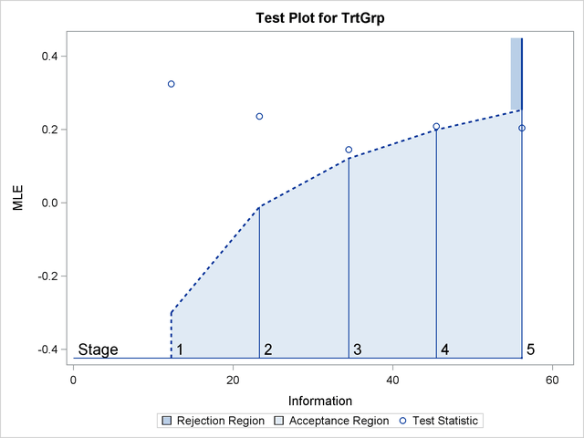
The "Test Information" table in Output 81.5.14 displays the boundary values for the test statistic with the specified MLE scale. The test statistic  is less than the corresponding upper boundary
  , so the sequential test stops to accept the null hypothesis. That is, there is no reduction in duration of symptoms for the group receiving vitamin C supplements.
| Test Information (MLE Scale) Null Reference = 0 |
||||||
|---|---|---|---|---|---|---|
| _Stage_ | Alternative | Boundary Values | Test | |||
| Information Level | Reference | Upper | TrtGrp | |||
| Proportion | Actual | Upper | Beta | Estimate | Action | |
| 1 | 0.2183 | 12.26014 | 0.44183 | -0.29906 | 0.32474 | Continue |
| 2 | 0.4145 | 23.27916 | 0.44183 | -0.01068 | 0.23560 | Continue |
| 3 | 0.6141 | 34.48793 | 0.44183 | 0.12134 | 0.14482 | Continue |
| 4 | 0.8092 | 45.44685 | 0.44183 | 0.19899 | 0.20855 | Continue |
| 5 | 1.0000 | 56.16068 | 0.44183 | 0.25375 | 0.20430 | Accept Null |
The "Test Plot" displays boundary values of the design and the test statistics, as shown in Output 81.5.15. It also shows that the test statistic is in the "Acceptance Region" at the final stage.
After a trial is stopped, the "Parameter Estimates" table in Output 81.5.16 displays the stopping stage, parameter estimate, unbiased median estimate, confidence limits, and the  -value under the null hypothesis
  . As expected, the -value
  is not significant at
  level and the lower
  confidence limit is less than the value
  . The -value, unbiased median estimate, and confidence limits depend on the ordering of the sample space
  , where
  is the stage number and
  is the standardized
  statistic.
| Parameter Estimates Stagewise Ordering |
|||||
|---|---|---|---|---|---|
| Parameter | Stopping Stage |
MLE | p-Value for H0:Parm=0 |
Median Estimate |
Lower 97.5% CL |
| TrtGrp | 5 | 0.204303 | 0.0456 | 0.234494 | -0.03712 |
Since the test is accepted at stage , the -value computed by using the default stagewise ordering can be expressed as
 |
where  is the test statistic at stage ,
  is a standardized normal variate at stage , and
  is the upper boundary value in the standardized scale at stage
  .
.
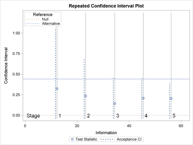
With the RCI option, the "Repeated Confidence Intervals" table in Output 81.5.17 displays repeated confidence intervals for the parameter. For a one-sided test with an upper alternative hypothesis, since the upper acceptance repeated confidence limit  at the final stage is less than the alternative reference
  , the null hypothesis is accepted.
| Repeated Confidence Intervals | |||
|---|---|---|---|
| _Stage_ | Information Level |
Parameter Estimate |
Acceptance Boundary |
| Upper 89.94% CL | |||
| 1 | 12.2601 | 0.32474 | 1.0656 |
| 2 | 23.2792 | 0.23560 | 0.6881 |
| 3 | 34.4879 | 0.14482 | 0.4653 |
| 4 | 45.4468 | 0.20855 | 0.4514 |
| 5 | 56.1607 | 0.20430 | 0.3924 |
With the PLOTS=RCI option, the "Repeated Confidence Intervals Plot" displays repeated confidence intervals for the parameter, as shown in Output 81.5.18. It shows that the upper acceptance repeated confidence limit at the final stage is less than the alternative reference . This implies that the study accepts the null hypothesis at the final stage.