The SEQTEST Procedure
- Overview
- Getting Started
-
Syntax

-
Details
Input Data Sets Boundary Variables Information Level Adjustments at Future Stages Boundary Adjustments for Information Levels Boundary Adjustments for Minimum Error Spending Boundary Adjustments for Overlapping Lower and Upper beta Boundaries Stochastic Curtailment Repeated Confidence Intervals Analysis after a Sequential Test Available Sample Space Orderings in a Sequential Test Applicable Tests and Sample Size Computation Table Output ODS Table Names Graphics Output ODS Graphics Acknowledgments
-
Examples
Testing the Difference between Two Proportions Testing an Effect in a Regression Model Testing an Effect with Early Stopping to Accept H0 Testing a Binomial Proportion Comparing Two Proportions with a Log Odds Ratio Test Comparing Two Survival Distributions with a Log-Rank Test Testing an Effect in a Proportional Hazards Regression Model Testing an Effect in a Logistic Regression Model
- References
Example 81.2 Testing an Effect in a Regression Model
This example demonstrates a two-sided group sequential test that uses an error spending design with early stopping to reject the null hypothesis. A study is conducted to examine the effects of Age (years), Weight (kg), RunTime (time in minutes to run 1.5 miles), RunPulse (heart rate while running), and MaxPulse (maximum heart rate recorded while running) on Oxygen (oxygen intake rate, ml per kg body weight per minute). The primary interest is whether oxygen intake rate is associated with weight.
The hypothesis is tested using the following linear model:
 |
The null hypothesis is  , where
  is the regression parameter for the variable Weight. Suppose that
  is the reference improvement that should be detected at a
  level. Then the maximum information
  can be derived in the SEQDESIGN procedure.
Following the derivations in the section "Test for a Parameter in the Regression Model" in the chapter "The SEQDESIGN Procedure," the required sample size can be derived from
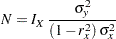 |
where  is the variance of the response variable in the regression model,
  is the proportion of variance of Weight explained by other covariates, and
  is the variance of Weight.
Further suppose that from past experience,  ,
,  , and
, and  . Then the required sample size can be derived using the SAMPLESIZE statement in the SEQDESIGN procedure.
The following statements invoke the SEQDESIGN procedure and request a three-stage group sequential design for normally distributed data to test the null hypothesis of a regression parameter against the alternative  :
:
ods graphics on;
proc seqdesign altref=0.10;
   OBFErrorFunction: design method=errfuncobf
                            nstages=3
                            info=cum(2 3 4)
                            ;
   samplesize model=reg(variance=5 xvariance=64 xrsquare=0.10);
ods output Boundary=Bnd_Fit;
run;
ods graphics off;
By default (or equivalently if you specify ALPHA=0.05 and BETA=0.10), the procedure uses a Type I error probability  and a Type II error probability
  . The ALTREF=0.10 option specifies a power of
  at the alternative hypothesis
  . The INFO=CUM(2 3 4) option specifies that the study perform the first interim analysis with information proportion
  —that is, after half of the total observations are collected.
The ODS OUTPUT statement with the BOUNDARY=BND_FIT option creates an output data set named BND_FIT which contains the resulting boundary information for the subsequent sequential tests.
The "Design Information" table in Output 81.2.1 displays design specifications and derived statistics. Since the alternative reference is specified, the maximum information is derived.
| Design Information | |
|---|---|
| Statistic Distribution | Normal |
| Boundary Scale | Standardized Z |
| Alternative Hypothesis | Two-Sided |
| Early Stop | Reject Null |
| Method | Error Spending |
| Boundary Key | Both |
| Alternative Reference | 0.1 |
| Number of Stages | 3 |
| Alpha | 0.05 |
| Beta | 0.1 |
| Power | 0.9 |
| Max Information (Percent of Fixed Sample) | 101.8276 |
| Max Information | 1069.948 |
| Null Ref ASN (Percent of Fixed Sample) | 101.2587 |
| Alt Ref ASN (Percent of Fixed Sample) | 77.81586 |
The "Boundary Information" table in Output 81.2.2 displays information level, alternative reference, and boundary values at each stage.
| Boundary Information (Standardized Z Scale) Null Reference = 0 |
|||||||
|---|---|---|---|---|---|---|---|
| _Stage_ | Alternative | Boundary Values | |||||
| Information Level | Reference | Lower | Upper | ||||
| Proportion | Actual | N | Lower | Upper | Alpha | Alpha | |
| 1 | 0.5000 | 534.9738 | 46.43869 | -2.31295 | 2.31295 | -2.96259 | 2.96259 |
| 2 | 0.7500 | 802.4606 | 69.65804 | -2.83277 | 2.83277 | -2.35902 | 2.35902 |
| 3 | 1.0000 | 1069.948 | 92.87739 | -3.27101 | 3.27101 | -2.01409 | 2.01409 |
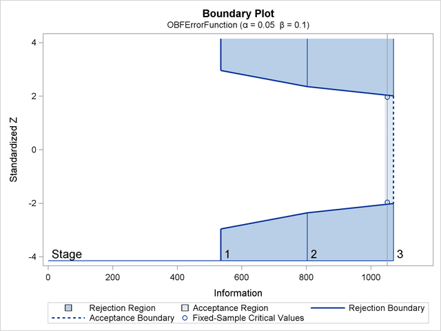
With ODS Graphics enabled, a detailed boundary plot with the rejection and acceptance regions is displayed, as shown in Output 81.2.3. The boundary plot also displays the information level and critical value for the corresponding fixed-sample design. This design has characteristics of an O’Brien-Fleming design; the probability for early stopping is low, and the maximum information and critical values at the final stage are similar to those of the corresponding fixed-sample design.
With the MODEL=REG option in the SAMPLESIZE statement, the "Sample Size Summary" table in Output 81.2.4 displays the parameters for the sample size computation.
| Sample Size Summary | |
|---|---|
| Test | Reg Parameter |
| Parameter | 0.1 |
| Variance | 5 |
| X Variance | 64 |
| R Square (X) | 0.1 |
| Max Sample Size | 92.87739 |
| Expected Sample Size (Null Ref) | 92.35845 |
| Expected Sample Size (Alt Ref) | 70.97617 |
The "Sample Sizes" table in Output 81.2.5 displays the required sample sizes for the group sequential clinical trial.
| Sample Sizes (N) Z Test for Regression Parameter |
||||
|---|---|---|---|---|
| _Stage_ | Fractional N | Ceiling N | ||
| N | Information | N | Information | |
| 1 | 46.44 | 535.0 | 47 | 541.4 |
| 2 | 69.66 | 802.5 | 70 | 806.4 |
| 3 | 92.88 | 1069.9 | 93 | 1071.4 |
Thus,  ,
,  , and
, and  individuals are needed in stages
  ,
,  , and
, and  , respectively. Since the sample sizes are derived from estimated values of , , and , the actual information levels might not achieve the target information levels. Thus, instead of specifying sample sizes in the protocol, you can specify the maximum information levels. Then if an actual information level is much less than the target level, you can increase the sample sizes for the remaining stages to achieve the desired information levels and power.
Suppose that individuals are available at stage . Output 81.2.6 lists the first  observations of the trial data.
| First 10 Obs in the Trial Data |
| Obs | Oxygen | Age | Weight | RunTime | RunPulse | MaxPulse |
|---|---|---|---|---|---|---|
| 1 | 54.5521 | 44 | 87.7676 | 11.6949 | 178.435 | 181.607 |
| 2 | 52.2821 | 40 | 75.4853 | 9.8872 | 184.433 | 183.667 |
| 3 | 62.1871 | 44 | 89.0638 | 8.7950 | 155.540 | 167.108 |
| 4 | 65.3269 | 42 | 67.7310 | 8.4577 | 162.926 | 173.877 |
| 5 | 59.9809 | 37 | 93.1902 | 9.3228 | 179.033 | 180.144 |
| 6 | 52.5588 | 47 | 75.9044 | 12.0385 | 177.753 | 175.033 |
| 7 | 51.7838 | 40 | 73.5422 | 11.6607 | 175.838 | 178.140 |
| 8 | 57.0024 | 43 | 81.2861 | 11.2219 | 160.963 | 171.770 |
| 9 | 48.0775 | 44 | 85.2290 | 13.1789 | 173.722 | 176.548 |
| 10 | 68.3357 | 38 | 80.2490 | 8.5066 | 171.824 | 184.011 |
The following statements use the REG procedure to estimate the slope and its associated standard error at stage :
proc reg data=Fit_1;
   model Oxygen=Age Weight RunTime RunPulse MaxPulse;
   ods output ParameterEstimates=Parms_Fit1;
run;
The following statements create and display (in Output 81.2.7) the input data set that contains slope and its associated standard error for the SEQTEST procedure:
data Parms_Fit1;
   set Parms_Fit1;
   if Variable='Weight';
   _Scale_='MLE';
   _Stage_= 1;
   keep _Scale_ _Stage_ Variable Estimate StdErr;
run;

proc print data=Parms_Fit1;
   title 'Statistics Computed at Stage 1';
run;
| Statistics Computed at Stage 1 |
| Obs | Variable | Estimate | StdErr | _Scale_ | _Stage_ |
|---|---|---|---|---|---|
| 1 | Weight | 0.03772 | 0.04345 | MLE | 1 |
The following statements invoke the SEQTEST procedure to test for early stopping at stage :
ods graphics on;
proc seqtest Boundary=Bnd_Fit
             Parms(Testvar=Weight)=Parms_Fit1
             infoadj=prop
             errspendadj=errfuncobf
             order=lr
             stopprob
             ;
ods output Test=Test_Fit1;
run;
ods graphics off;
The BOUNDARY= option specifies the input data set that provides the boundary information for the trial at stage (this data set was generated in the SEQDESIGN procedure). Recall that these boundary values were derived for the information levels specified with the INFO=CUM(2 3 4) option in the SEQDESIGN procedure. The PARMS=PARMS_FIT1 option specifies the input data set PARMS_FIT1 that contains the test statistic and its associated standard error at stage , and the TESTVAR=WEIGHT option identifies the test variable WEIGHT in the data set.
If the computed information level for stage is not the same as the value provided in the BOUNDARY= data set, the INFOADJ=PROP option (which is the default) proportionally adjusts the information levels at future interim stages from the levels provided in the BOUNDARY= data set. The ORDER=LR option uses the LR ordering to derive the  -value, the unbiased median estimate, and the confidence limits for the regression slope estimate. The ERRSPENDADJ=ERRFUNCOBF option adjusts the boundaries with the updated error spending values generated from an O’Brien-Fleming-type cumulative error spending function.
The ODS OUTPUT statement with the TEST=TEST_FIT1 option creates an output data set named TEST_FIT1 which contains the updated boundary information for the test at stage . The adjustment is needed because the observed information level is different from the information level in the BOUNDARY= data set. The data set TEST_FIT1 also provides the boundary information that is needed for the group sequential test at the next stage.
The "Design Information" table in Output 81.2.8 displays the design specifications. By default (or equivalently if you specify BOUNDARYKEY=ALPHA), the boundary values are modified for the new information levels to maintain the Type I  level. The maximum information remains the same as in the BOUNDARY= data set, but the derived Type II error probability
  and power
  are different because of the new information level.
| Design Information | |
|---|---|
| BOUNDARY Data Set | WORK.BND_FIT |
| Data Set | WORK.PARMS_FIT1 |
| Statistic Distribution | Normal |
| Boundary Scale | Standardized Z |
| Alternative Hypothesis | Two-Sided |
| Early Stop | Reject Null |
| Number of Stages | 3 |
| Alpha | 0.05 |
| Beta | 0.09994 |
| Power | 0.90006 |
| Max Information (Percent of Fixed Sample) | 101.8057 |
| Max Information | 1069.94751 |
| Null Ref ASN (Percent of Fixed Sample) | 101.2416 |
| Alt Ref ASN (Percent of Fixed Sample) | 77.87607 |
With the STOPPROB option, the "Expected Cumulative Stopping Probabilities" table in Output 81.2.9 displays the expected stopping stage and cumulative stopping probability to reject the null hypothesis at each stage under various hypothetical references  , where
  is the alternative reference and
  by default. You can specify other values for
  with the CREF= option.
| Expected Cumulative Stopping Probabilities Reference = CRef * (Alt Reference) |
|||||
|---|---|---|---|---|---|
| CRef | Expected Stopping Stage |
Source | Stopping Probabilities | ||
| Stage_1 | Stage_2 | Stage_3 | |||
| 0.0000 | 2.978 | Reject Null | 0.00289 | 0.01906 | 0.05000 |
| 0.5000 | 2.792 | Reject Null | 0.03373 | 0.17443 | 0.36566 |
| 1.0000 | 2.069 | Reject Null | 0.24884 | 0.68206 | 0.90006 |
| 1.5000 | 1.348 | Reject Null | 0.68172 | 0.97032 | 0.99820 |
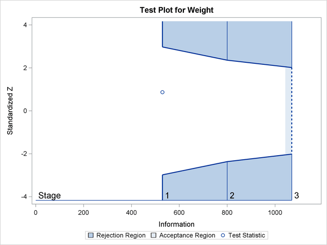
The "Test Information" table in Output 81.2.10 displays the boundary values for the test statistic. By default (or equivalently if you specify BOUNDARYSCALE=STDZ), these statistics are displayed with the standardized  scale. The information level at stage is derived from the standard error
  in the PARMS= data set,
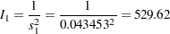 |
| Test Information (Standardized Z Scale) Null Reference = 0 |
||||||||
|---|---|---|---|---|---|---|---|---|
| _Stage_ | Alternative | Boundary Values | Test | |||||
| Information Level | Reference | Lower | Upper | Weight | ||||
| Proportion | Actual | Lower | Upper | Alpha | Alpha | Estimate | Action | |
| 1 | 0.4950 | 529.6232 | -2.30135 | 2.30135 | -2.97951 | 2.97951 | 0.86798 | Continue |
| 2 | 0.7475 | 799.7853 | -2.82805 | 2.82805 | -2.36291 | 2.36291 | . | |
| 3 | 1.0000 | 1069.948 | -3.27101 | 3.27101 | -2.01336 | 2.01336 | . | |
With the INFOADJ=PROP option (which is the default), the information level at stage is derived proportionally from the observed information at stage and the information levels in the BOUNDARY= data set. See the section Boundary Adjustments for Information Levels for details about how the adjusted information levels are computed.
At stage , the standardized statistic  is between the lower boundary
  and the upper boundary
  , so the trial continues to the next stage.
With ODS Graphics enabled, a boundary plot with test statistics is displayed, as shown in Output 81.2.11. As expected, the test statistic is in the continuation region between the lower and upper boundaries.
The following statements use the REG procedure to estimate the slope and its associated standard error at stage :
proc reg data=Fit_2;
   model Oxygen=Age Weight RunTime RunPulse MaxPulse;
   ods output ParameterEstimates=Parms_Fit2;
run;
Note that the data set Fit_2 contains both the data from stage and the data from stage .
The following statements create and display (in Output 81.2.12) the input data set that contains slope and its associated standard error at stage for the SEQTEST procedure:
data Parms_Fit2;
   set Parms_Fit2;
   if Variable='Weight';
   _Scale_='MLE';
   _Stage_= 2;
   keep _Scale_ _Stage_ Variable Estimate StdErr;
run;


proc print data=Parms_Fit2;
   title 'Statistics Computed at Stage 2';
run;
| Statistics Computed at Stage 2 |
| Obs | Variable | Estimate | StdErr | _Scale_ | _Stage_ |
|---|---|---|---|---|---|
| 1 | Weight | 0.02932 | 0.03520 | MLE | 2 |
The following statements invoke the SEQTEST procedure to test for early stopping at stage :
proc seqtest Boundary=Test_Fit1
             Parms(Testvar=Weight)=Parms_Fit2
             infoadj=prop
             errspendadj=errfuncobf
             order=lr
             ;
ods output Test=Test_Fit2;
run;
The BOUNDARY= option specifies the input data set that provides the boundary information for the trial at stage , which was generated by the SEQTEST procedure at the previous stage. The PARMS= option specifies the input data set that contains the test statistic and its associated standard error at stage , and the TESTVAR= option identifies the test variable in the data set.
The ODS OUTPUT statement with the TEST=TEST_FIT2 option creates an output data set named TEST_FIT2 which contains the updated boundary information for the test at stage . The data set also provides the boundary information that is needed for the group sequential test at the next stage.
Since the data set PARMS_FIT2 does not contain the test information at stage , the information level at stage in the TEST_FIT1 data set is used to generate boundary values for the test at stage .
Following the process at stage , the slope estimate is also between its corresponding lower and upper boundary values, so the trial continues to the next stage.
The following statements use the REG procedure to estimate the slope and its associated standard error at the final stage:
proc reg data=Fit_3;
   model Oxygen=Age Weight RunTime RunPulse MaxPulse;
   ods output ParameterEstimates=Parms_Fit3;
run;
The following statements create the input data set that contains slope and its associated standard error at stage for the SEQTEST procedure:
data Parms_Fit3;
   set Parms_Fit3;
   if Variable='Weight';
   _Scale_='MLE';
   _Stage_= 3;
   keep _Scale_ _Stage_ Variable Estimate StdErr;
run;
The following statements print (in Output 81.2.13) the test statistics at stage :
proc print data=Parms_Fit3;
   title 'Statistics Computed at Stage 3';
run;
| Statistics Computed at Stage 3 |
| Obs | Variable | Estimate | StdErr | _Scale_ | _Stage_ |
|---|---|---|---|---|---|
| 1 | Weight | 0.02189 | 0.03028 | MLE | 3 |
The following statements invoke the SEQTEST procedure to test the hypothesis:
ods graphics on;
proc seqtest Boundary=Test_Fit2
             Parms(testvar=Weight)=Parms_Fit3
             errspendadj=errfuncobf
             order=lr
             pss
             plots=(asn power)
             ;
ods output Test=Test_Fit3;
run;
ods graphics off;
The BOUNDARY= option specifies the input data set that provides the boundary information for the trial at stage , which was generated by the SEQTEST procedure at the previous stage. The PARMS= option specifies the input data set that contains the test statistic and its associated standard error at stage , and the TESTVAR= option identifies the test variable in the data set.
The ODS OUTPUT statement with the TEST=TEST_FIT3 option creates an output data set named TEST_FIT3 which contains the updated boundary information for the test at stage .
The "Design Information" table in Output 81.2.14 displays design specifications. By default (or equivalently if you specify BOUNDARYKEY=ALPHA), the boundary values are modified for the new information levels to maintain the Type I level.
| Design Information | |
|---|---|
| BOUNDARY Data Set | WORK.TEST_FIT2 |
| Data Set | WORK.PARMS_FIT3 |
| Statistic Distribution | Normal |
| Boundary Scale | Standardized Z |
| Alternative Hypothesis | Two-Sided |
| Early Stop | Reject Null |
| Number of Stages | 3 |
| Alpha | 0.05 |
| Beta | 0.09514 |
| Power | 0.90486 |
| Max Information (Percent of Fixed Sample) | 102.0102 |
| Max Information | 1090.63724 |
| Null Ref ASN (Percent of Fixed Sample) | 101.4122 |
| Alt Ref ASN (Percent of Fixed Sample) | 77.22139 |
The maximum information is derived from the standard error associated with the slope estimate at the final stage and is larger than the target level. The derived Type II error probability and power are different because of the new information levels.
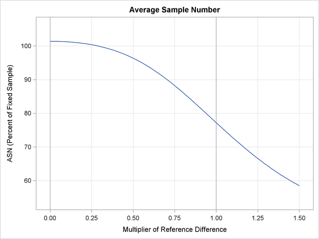
With the PSS option, the "Power and Expected Sample Sizes" table in Output 81.2.15 displays powers and expected mean sample sizes under various hypothetical references , where is the alternative reference and by default. You can specify the values with the CREF= option.
| Powers and Expected Sample Sizes Reference = CRef * (Alt Reference) |
||
|---|---|---|
| CRef | Power | Sample Size |
| Percent Fixed-Sample |
||
| 0.0000 | 0.02500 | 101.4122 |
| 0.5000 | 0.37046 | 96.3754 |
| 1.0000 | 0.90486 | 77.2214 |
| 1.5000 | 0.99844 | 58.5301 |
With the PLOTS=ASN option, the procedure displays a plot of expected sample sizes under various hypothetical references, as shown in Output 81.2.16. By default, expected sample sizes under the hypotheses  ,
,  , are displayed, where is the alternative reference.
With the PLOTS=POWER option, the procedure displays a plot of powers under various hypothetical references, as shown in Output 81.2.17. By default, powers under hypothetical references are displayed, where by default. You can specify values with the CREF= option. The values are displayed on the horizontal axis.
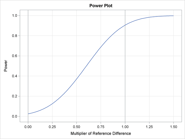
Under the null hypothesis,  , the power is
  , which is the upper Type I error probability. Under the alternative hypothesis,
  , the power is
  , which is one minus the Type II error probability.
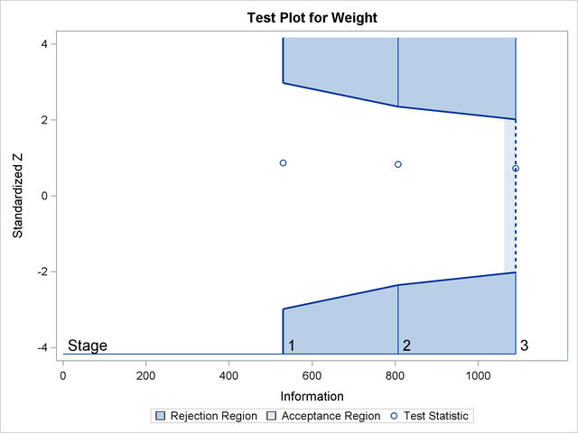
The "Test Information" table in Output 81.2.18 displays the boundary values for the test statistic with the default standardized scale. The information level at the current stage is derived from the standard error for the current stage in the PARMS= data set. At stage , the standardized slope estimate  is still between the lower and upper boundary values. Since it is the final stage, the trial stops to accept the null hypothesis that the variable Weight has no effect on the oxygen intake rate after adjusting for other covariates.
| Test Information (Standardized Z Scale) Null Reference = 0 |
||||||||
|---|---|---|---|---|---|---|---|---|
| _Stage_ | Alternative | Boundary Values | Test | |||||
| Information Level | Reference | Lower | Upper | Weight | ||||
| Proportion | Actual | Lower | Upper | Alpha | Alpha | Estimate | Action | |
| 1 | 0.4856 | 529.6232 | -2.30135 | 2.30135 | -2.97951 | 2.97951 | 0.86798 | Continue |
| 2 | 0.7401 | 807.1954 | -2.84112 | 2.84112 | -2.34945 | 2.34945 | 0.83305 | Continue |
| 3 | 1.0000 | 1090.637 | -3.30248 | 3.30248 | -2.01885 | 2.01885 | 0.72284 | Accept Null |
Since the data set FIT_3 contains the test information only at stage , the information levels at previous stages in the TEST_FIT2 data set are used to generate boundary values for the test.
With ODS Graphics enabled, a boundary plot with test statistics is displayed, as shown in Output 81.2.19. As expected, the test statistic is in the acceptance region between the lower and upper boundaries at the final stage.
After a trial is stopped, the "Parameter Estimates" table in Output 81.2.20 displays the stopping stage, parameter estimate, unbiased median estimate, confidence limits, and the -value under the null hypothesis  .
.
| Parameter Estimates LR Ordering |
||||||
|---|---|---|---|---|---|---|
| Parameter | Stopping Stage |
MLE | p-Value for H0:Parm=0 |
Median Estimate |
95% Confidence Limits | |
| Weight | 3 | 0.021888 | 0.4699 | 0.021884 | -0.03747 | 0.08123 |
As expected, the -value  is not significant at the
  level, and the confidence interval does contain the value zero. The -value, unbiased median estimate, and confidence limits depend on the ordering of the sample space
  , where
  is the stage number and
  is the standardized statistic. With the specified LR ordering, the -values are computed with the ordering
  if
if  . See the section Available Sample Space Orderings in a Sequential Test for a detailed description of the LR ordering.