The SEQDESIGN Procedure
-
Overview

- Getting Started
-
Syntax
-
Details
Fixed-Sample Clinical Trials One-Sided Fixed-Sample Tests in Clinical Trials Two-Sided Fixed-Sample Tests in Clinical Trials Group Sequential Methods Statistical Assumptions for Group Sequential Designs Boundary Scales Boundary Variables Type I and Type II Errors Unified Family Methods Haybittle-Peto Method Whitehead Methods Error Spending Methods Acceptance (beta) Boundary Boundary Adjustments for Overlapping Lower and Upper beta Boundaries Specified and Derived Parameters Applicable Boundary Keys Sample Size Computation Applicable One-Sample Tests and Sample Size Computation Applicable Two-Sample Tests and Sample Size Computation Applicable Regression Parameter Tests and Sample Size Computation Aspects of Group Sequential Designs Summary of Methods in Group Sequential Designs Table Output ODS Table Names Graphics Output ODS Graphics Acknowledgments
-
Examples
Creating Fixed-Sample Designs Creating a One-Sided O’Brien-Fleming Design Creating Two-Sided Pocock and O’Brien-Fleming Designs Generating Graphics Display for Sequential Designs Creating Designs Using Haybittle-Peto Methods Creating Designs with Various Stopping Criteria Creating Whitehead’s Triangular Designs Creating a One-Sided Error Spending Design Creating Designs with Various Number of Stages Creating Two-Sided Error Spending Designs with and without Overlapping Lower and Upper beta Boundaries Creating a Two-Sided Asymmetric Error Spending Design with Early Stopping to Reject H0 Creating a Two-Sided Asymmetric Error Spending Design with Early Stopping to Reject or Accept H0
- References
Example 80.11 Creating a Two-Sided Asymmetric Error Spending Design with Early Stopping to Reject H0
This example requests a three-stage two-sided asymmetric group sequential design for normally distributed statistics.
The O’Brien-Fleming boundary can be approximated using a power family error spending function with parameter  , and the Pocock boundary can be approximated using a power family error spending function with parameter
  (Jennison and Turnbull 2000, p. 148). The following statements use the power family error spending function to creates a two-sided asymmetric design with early stopping to reject the null hypothesis
  :
:
ods graphics on;
proc seqdesign altref=1.0
               pss(cref=0 0.5 1)
               stopprob(cref=0 0.5 1)
               errspend
               plots=(asn power errspend)
               ;

   TwoSidedErrorSpending: design nstages=3
                          method(upperalpha)=errfuncpow(rho=3)
                          method(loweralpha)=errfuncpow(rho=1)
                          info=cum(2 3 4)
                          alt=twosided
                          stop=reject
                          alpha=0.075(upper=0.025)
                          ;
run;
ods graphics off;
The design uses power family error spending functions with for the lower  boundary and for the upper boundary. Thus, the design is conservative in the early stages and tends to stop the trials early only with a small
  -value for the upper boundary. The upper level
  is specified explicitly, and the lower level is computed as
  .
.
The "Design Information" table in Output 80.11.1 displays design specifications and the derived maximum information. Note that in order to attain the same information level for the asymmetric lower and upper boundaries, the derived power at the lower alternative  is larger than the default
  .
.
| Design Information | |
|---|---|
| Statistic Distribution | Normal |
| Boundary Scale | Standardized Z |
| Alternative Hypothesis | Two-Sided |
| Early Stop | Reject Null |
| Method | Error Spending |
| Boundary Key | Both |
| Alternative Reference | 1 |
| Number of Stages | 3 |
| Alpha | 0.075 |
| Alpha (Lower) | 0.05 |
| Alpha (Upper) | 0.025 |
| Beta (Lower) | 0.07037 |
| Beta (Upper) | 0.1 |
| Power (Lower) | 0.92963 |
| Power (Upper) | 0.9 |
| Max Information (Percent of Fixed Sample) | 102.4384 |
| Max Information | 10.76365 |
| Null Ref ASN (Percent of Fixed Sample) | 100.4877 |
| Lower Alt Ref ASN (Percent of Fixed Sample) | 64.8288 |
| Upper Alt Ref ASN (Percent of Fixed Sample) | 75.98778 |
The "Method Information" table in Output 80.11.2 displays the specified and  error levels and the derived drift parameter. With the same information level used for the asymmetric lower and upper boundaries, only one of the levels is maintained, and the other is derived to have the level less than or equal to the default level.
| Method Information | ||||||
|---|---|---|---|---|---|---|
| Boundary | Method | Alpha | Beta | Error Spending | Alternative Reference |
Drift |
| Function | ||||||
| Upper Alpha | Error Spending | 0.02500 | 0.10000 | Power (Rho=3) | 1 | 3.280801 |
| Lower Alpha | Error Spending | 0.05000 | 0.07037 | Power (Rho=1) | -1 | -3.2808 |
With the STOPPROB(CREF=0 0.5 1) option, the "Expected Cumulative Stopping Probabilities" table in Output 80.11.3 displays the expected stopping stage and cumulative stopping probability to reject the null hypothesis  at each stage under hypothetical references
  (null hypothesis ),
  , and
, and  (alternative hypothesis
  ), where
  is the alternative reference.
| Expected Cumulative Stopping Probabilities Reference = CRef * (Alt Reference) |
||||||
|---|---|---|---|---|---|---|
| CRef | Ref | Expected Stopping Stage |
Source | Stopping Probabilities | ||
| Stage_1 | Stage_2 | Stage_3 | ||||
| 0.0000 | Lower Alt | 2.924 | Rej Null (Lower Alt) | 0.02500 | 0.03750 | 0.05000 |
| 0.0000 | Lower Alt | 2.924 | Rej Null (Upper Alt) | 0.00313 | 0.01055 | 0.02500 |
| 0.0000 | Lower Alt | 2.924 | Reject Null | 0.02813 | 0.04805 | 0.07500 |
| 0.5000 | Lower Alt | 2.456 | Rej Null (Lower Alt) | 0.21185 | 0.33190 | 0.45370 |
| 0.5000 | Lower Alt | 2.456 | Rej Null (Upper Alt) | 0.00005 | 0.00012 | 0.00021 |
| 0.5000 | Lower Alt | 2.456 | Reject Null | 0.21190 | 0.33202 | 0.45391 |
| 1.0000 | Lower Alt | 1.531 | Rej Null (Lower Alt) | 0.64054 | 0.82803 | 0.92963 |
| 1.0000 | Lower Alt | 1.531 | Rej Null (Upper Alt) | 0.00000 | 0.00000 | 0.00000 |
| 1.0000 | Lower Alt | 1.531 | Reject Null | 0.64054 | 0.82803 | 0.92963 |
| 0.0000 | Upper Alt | 2.924 | Rej Null (Lower Alt) | 0.02500 | 0.03750 | 0.05000 |
| 0.0000 | Upper Alt | 2.924 | Rej Null (Upper Alt) | 0.00313 | 0.01055 | 0.02500 |
| 0.0000 | Upper Alt | 2.924 | Reject Null | 0.02813 | 0.04805 | 0.07500 |
| 0.5000 | Upper Alt | 2.758 | Rej Null (Lower Alt) | 0.00090 | 0.00110 | 0.00120 |
| 0.5000 | Upper Alt | 2.758 | Rej Null (Upper Alt) | 0.05769 | 0.18269 | 0.36458 |
| 0.5000 | Upper Alt | 2.758 | Reject Null | 0.05860 | 0.18379 | 0.36578 |
| 1.0000 | Upper Alt | 1.967 | Rej Null (Lower Alt) | 0.00001 | 0.00001 | 0.00001 |
| 1.0000 | Upper Alt | 1.967 | Rej Null (Upper Alt) | 0.33926 | 0.69356 | 0.90000 |
| 1.0000 | Upper Alt | 1.967 | Reject Null | 0.33927 | 0.69357 | 0.90001 |
"Rej Null (Lower Alt)" and "Rej Null (Upper Alt)" under the heading "Source" indicate the probabilities of rejecting the null hypothesis for the lower alternative and for the upper alternative, respectively. "Reject Null" indicates the probability of rejecting the null hypothesis for either the lower or upper alternative.
Note that with the STOP=REJECT option, the cumulative stopping probability of accepting the null hypothesis at each interim stage is zero and is not displayed.
With the PSS(CREF=0 0.5 1.0) option, the "Power and Expected Sample Sizes" table in Output 80.11.4 displays powers and expected sample sizes under hypothetical references (null hypothesis ), , and (alternative hypothesis ), where is the alternative reference. The expected sample sizes are displayed in a percentage scale relative to the corresponding fixed-sample size design.
| Powers and Expected Sample Sizes Reference = CRef * (Alt Reference) |
|||
|---|---|---|---|
| CRef | Ref | Power | Sample Size |
| Percent Fixed-Sample |
|||
| 0.0000 | Lower Alt | 0.05000 | 100.4877 |
| 0.5000 | Lower Alt | 0.45370 | 88.5090 |
| 1.0000 | Lower Alt | 0.92963 | 64.8288 |
| 0.0000 | Upper Alt | 0.02500 | 100.4877 |
| 0.5000 | Upper Alt | 0.36458 | 96.2309 |
| 1.0000 | Upper Alt | 0.90000 | 75.9878 |
Note that at  , the null reference
  , the power with the lower alternative is the lower error
  , and the power with the upper alternative is the upper error . At
  , the alternative reference
  , the power with the upper alternative is the specified power , and the power with the lower alternative is greater than the specified power because the same information level is used for these two asymmetric boundaries.
With the PLOTS=POWER option, the procedure displays a plot of the power curves under various hypothetical references, as shown in Output 80.11.5. By default, powers under the lower hypotheses  and under the upper hypotheses
  are displayed for a two-sided asymmetric design, where
  and
and  and
and  are the lower and upper alternative references, respectively.
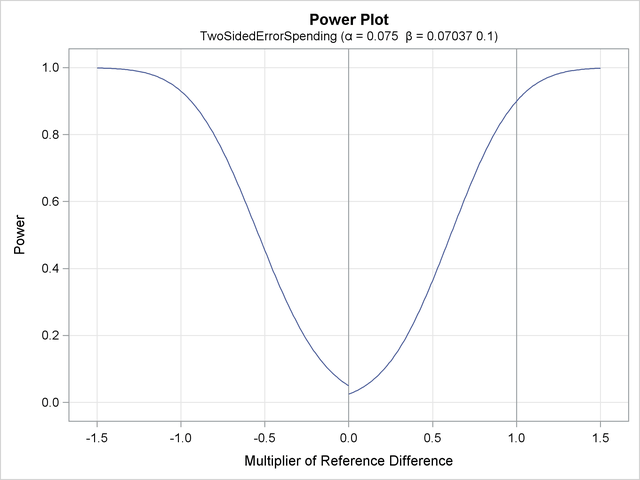
The horizontal axis displays the multiplier of the reference difference. A positive multiplier corresponds to  for the upper alternative hypothesis, and a negative multiplier corresponds to
  for the lower alternative hypothesis. For lower reference hypotheses, the power is the lower error under the null hypothesis () and is under the alternative hypothesis (). For upper reference hypotheses, the power is the upper error under the null hypothesis () and is under the alternative hypothesis ().
With the PLOTS=ASN option, the procedure displays a plot of expected sample sizes under various hypothetical references, as shown in Output 80.11.6. By default, expected sample sizes under the lower hypotheses and under the upper hypotheses , , are displayed for a two-sided asymmetric design, where and are the lower and upper alternative references, respectively.
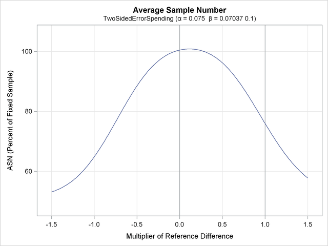
The horizontal axis displays the multiplier of the reference difference. A positive multiplier corresponds to for the upper alternative hypothesis and a negative multiplier corresponds to for the lower alternative hypothesis.
The "Boundary Information" table in Output 80.11.7 displays the information levels, alternative references, and boundary values. By default (or equivalently if you specify BOUNDARYSCALE=STDZ), the standardized  scale is used to display the alternative references and boundary values. The resulting standardized alternative references at stage
  are given by
  , where
  is the specified alternative reference and
  is the information level at stage ,
  .
.
| Boundary Information (Standardized Z Scale) Null Reference = 0 |
||||||
|---|---|---|---|---|---|---|
| _Stage_ | Alternative | Boundary Values | ||||
| Information Level | Reference | Lower | Upper | |||
| Proportion | Actual | Lower | Upper | Alpha | Alpha | |
| 1 | 0.5000 | 5.381827 | -2.31988 | 2.31988 | -1.95996 | 2.73437 |
| 2 | 0.7500 | 8.07274 | -2.84126 | 2.84126 | -1.98394 | 2.35681 |
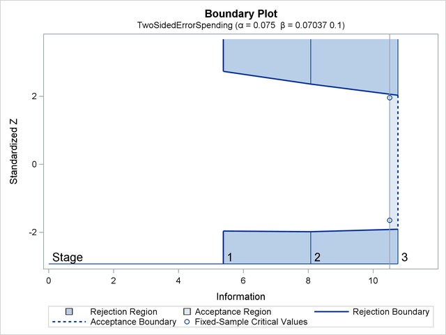
| 3 | 1.0000 | 10.76365 | -3.28080 | 3.28080 | -1.90855 | 2.02853 |
With ODS Graphics enabled, a detailed boundary plot with the rejection and acceptance regions is displayed, as shown in Output 80.11.8.
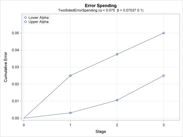
The "Error Spending Information" table in Output 80.11.9 displays the cumulative error spending at each stage for each boundary.
| Error Spending Information | |||||
|---|---|---|---|---|---|
| _Stage_ | Information Level |
Cumulative Error Spending | |||
| Lower | Upper | ||||
| Proportion | Alpha | Beta | Beta | Alpha | |
| 1 | 0.5000 | 0.02500 | 0.00000 | 0.00001 | 0.00313 |
| 2 | 0.7500 | 0.03750 | 0.00000 | 0.00001 | 0.01055 |
| 3 | 1.0000 | 0.05000 | 0.07037 | 0.10000 | 0.02500 |
With the STOP=REJECT option, there is no early stopping to accept , and the corresponding spending at an interim stage is computed from the rejection region. For example, the upper spending at stage  (
( ) is the probability of rejecting for the lower alternative under the upper alternative reference.
With the PLOTS=ERRSPEND option, the procedure displays a plot of the cumulative error spending on each boundary at each stage, as shown in Output 80.11.10.