The SEQDESIGN Procedure
-
Overview

- Getting Started
-
Syntax
-
Details
Fixed-Sample Clinical Trials One-Sided Fixed-Sample Tests in Clinical Trials Two-Sided Fixed-Sample Tests in Clinical Trials Group Sequential Methods Statistical Assumptions for Group Sequential Designs Boundary Scales Boundary Variables Type I and Type II Errors Unified Family Methods Haybittle-Peto Method Whitehead Methods Error Spending Methods Acceptance (beta) Boundary Boundary Adjustments for Overlapping Lower and Upper beta Boundaries Specified and Derived Parameters Applicable Boundary Keys Sample Size Computation Applicable One-Sample Tests and Sample Size Computation Applicable Two-Sample Tests and Sample Size Computation Applicable Regression Parameter Tests and Sample Size Computation Aspects of Group Sequential Designs Summary of Methods in Group Sequential Designs Table Output ODS Table Names Graphics Output ODS Graphics Acknowledgments
-
Examples
Creating Fixed-Sample Designs Creating a One-Sided O’Brien-Fleming Design Creating Two-Sided Pocock and O’Brien-Fleming Designs Generating Graphics Display for Sequential Designs Creating Designs Using Haybittle-Peto Methods Creating Designs with Various Stopping Criteria Creating Whitehead’s Triangular Designs Creating a One-Sided Error Spending Design Creating Designs with Various Number of Stages Creating Two-Sided Error Spending Designs with and without Overlapping Lower and Upper beta Boundaries Creating a Two-Sided Asymmetric Error Spending Design with Early Stopping to Reject H0 Creating a Two-Sided Asymmetric Error Spending Design with Early Stopping to Reject or Accept H0
- References
Example 80.9 Creating Designs with Various Number of Stages
This example requests three group sequential designs for normally distributed statistics. Each design uses the power family error spending function with the default power parameter  . The specified error spending method is between the approximated Pocock method (
 ) and the approximated O’Brien-Fleming method (
 ) (Jennison and Turnbull 1999, p. 148). The three designs are identical except for the specified number of stages. The following statements request these three group sequential designs:
ods graphics on;
proc seqdesign plots=( asn
                       power
                       combinedboundary
                       errspend(hscale=info)
                       )
               ;
   TwoStageDesign:  design nstages=2
                    method=errfuncpow
                    alt=upper  stop=reject
                    ;
   FiveStageDesign: design nstages=5
                    method=errfuncpow
                    alt=upper  stop=reject
                    ;
   TenStageDesign:  design nstages=10
                    method=errfuncpow
                    alt=upper  stop=reject
                    ;
run;
ods graphics off;
The "Design Information" table in Output 80.9.1 displays design information for the two-stage design.
| Design Information | |
|---|---|
| Statistic Distribution | Normal |
| Boundary Scale | Standardized Z |
| Alternative Hypothesis | Upper |
| Early Stop | Reject Null |
| Method | Error Spending |
| Boundary Key | Both |
| Number of Stages | 2 |
| Alpha | 0.05 |
| Beta | 0.1 |
| Power | 0.9 |
| Max Information (Percent of Fixed Sample) | 102.4167 |
| Null Ref ASN (Percent of Fixed Sample) | 101.7766 |
| Alt Ref ASN (Percent of Fixed Sample) | 79.81021 |
The "Boundary Information" table in Output 80.9.2 displays the information level, alternative reference, and boundary values. By default (or equivalently if you specify BOUNDARYSCALE=STDZ), the alternative reference and boundary values are displayed with the standardized normal  scale. The resulting standardized alternative reference at stage
  is given by
  , where
  is the alternative reference and
  is the information level at stage ,
  .
.
 Scale
Scale
| Boundary Information (Standardized Z Scale) Null Reference = 0 |
|||
|---|---|---|---|
| _Stage_ | Information Level |
Alternative | Boundary Values |
| Reference | Upper | ||
| Proportion | Upper | Alpha | |
| 1 | 0.5000 | 2.09414 | 2.24140 |
| 2 | 1.0000 | 2.96156 | 1.69970 |
The "Design Information" table in Output 80.9.3 displays design information for the five-stage design. Compared with the two-stage design in Output 80.9.1, the maximum information increases from  to
to  , and the average sample number under the alternative reference (Alt Ref ASN) decreases from
  to
to  .
.
| Design Information | |
|---|---|
| Statistic Distribution | Normal |
| Boundary Scale | Standardized Z |
| Alternative Hypothesis | Upper |
| Early Stop | Reject Null |
| Method | Error Spending |
| Boundary Key | Both |
| Number of Stages | 5 |
| Alpha | 0.05 |
| Beta | 0.1 |
| Power | 0.9 |
| Max Information (Percent of Fixed Sample) | 105.6235 |
| Null Ref ASN (Percent of Fixed Sample) | 104.356 |
| Alt Ref ASN (Percent of Fixed Sample) | 69.64322 |
The "Boundary Information" table in Output 80.9.4 displays the information level, alternative reference, and boundary values with the default standardized normal scale.
Scale
| Boundary Information (Standardized Z Scale) Null Reference = 0 |
|||
|---|---|---|---|
| _Stage_ | Information Level |
Alternative | Boundary Values |
| Reference | Upper | ||
| Proportion | Upper | Alpha | |
| 1 | 0.2000 | 1.34502 | 2.87816 |
| 2 | 0.4000 | 1.90215 | 2.47023 |
| 3 | 0.6000 | 2.32965 | 2.20095 |
| 4 | 0.8000 | 2.69005 | 1.98182 |
| 5 | 1.0000 | 3.00756 | 1.79024 |
The "Design Information" table in Output 80.9.5 displays design information for the ten-stage design. Compared with the five-stage design in Output 80.9.3, the maximum information increases further from to  and under the alternative reference, the average sample number decreases further from to
  .
.
| Design Information | |
|---|---|
| Statistic Distribution | Normal |
| Boundary Scale | Standardized Z |
| Alternative Hypothesis | Upper |
| Early Stop | Reject Null |
| Method | Error Spending |
| Boundary Key | Both |
| Number of Stages | 10 |
| Alpha | 0.05 |
| Beta | 0.1 |
| Power | 0.9 |
| Max Information (Percent of Fixed Sample) | 107.256 |
| Null Ref ASN (Percent of Fixed Sample) | 105.7276 |
| Alt Ref ASN (Percent of Fixed Sample) | 66.35565 |
The "Boundary Information" table in Output 80.9.6 displays the information level, alternative reference, and boundary values with the default standardized normal scale.
Scale
| Boundary Information (Standardized Z Scale) Null Reference = 0 |
|||
|---|---|---|---|
| _Stage_ | Information Level |
Alternative | Boundary Values |
| Reference | Upper | ||
| Proportion | Upper | Alpha | |
| 1 | 0.1000 | 0.95840 | 3.29053 |
| 2 | 0.2000 | 1.35538 | 2.94037 |
| 3 | 0.3000 | 1.65999 | 2.72115 |
| 4 | 0.4000 | 1.91679 | 2.54808 |
| 5 | 0.5000 | 2.14304 | 2.40114 |
| 6 | 0.6000 | 2.34758 | 2.27127 |
| 7 | 0.7000 | 2.53568 | 2.15359 |
| 8 | 0.8000 | 2.71076 | 2.04503 |
| 9 | 0.9000 | 2.87519 | 1.94355 |
| 10 | 1.0000 | 3.03072 | 1.84765 |
With the PLOTS=ASN option, the procedure displays a plot of average sample numbers under various hypothetical references for all designs simultaneously, as shown in Output 80.9.7. By default, the option CREF= 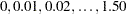 and expected sample sizes under the hypothetical references
  are displayed, where
  are values specified in the CREF= option. These CREF= values are displayed on the horizontal axis.
The plot shows that as the number of stages increases, the average sample number as a percentage of the fixed-sample design increases under the null hypothesis ( ) but decreases under the alternative hypothesis (
 ).
).
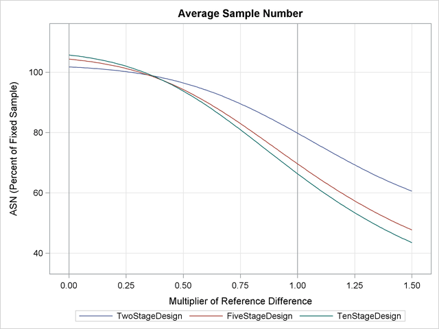
With the PLOTS=POWER option, the procedure displays a plot of the power curves under various hypothetical references for all designs simultaneously, as shown in Output 80.9.8. By default, the option CREF= and powers under hypothetical references are displayed, where are values specified in the CREF= option. These CREF= values are displayed on the horizontal axis.
Under the null hypothesis, , the power is  , the upper Type I error probability. Under the alternative hypothesis, , the power is
  , one minus the Type II error probability. The plot shows only minor difference among the three designs.
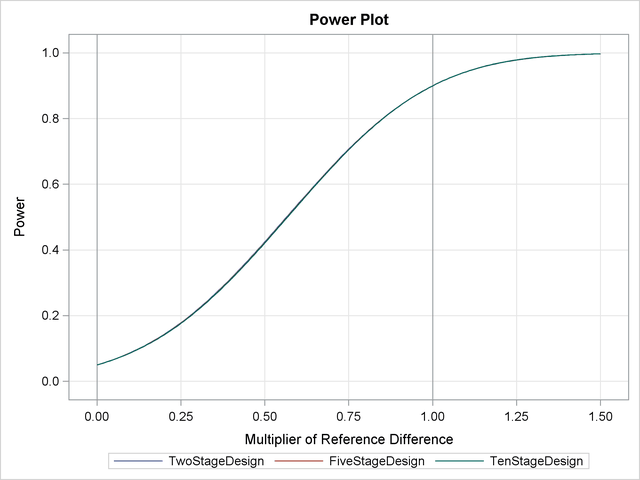
With the PLOTS=COMBINEDBOUNDARY option, the procedure displays a plot of sequential boundaries for all designs simultaneously, as shown in Output 80.9.9. By default (or equivalently if you specify COMBINEDBOUNDARY(HSCALE=INFO)), the information levels are used on the horizontal axis. Since the maximum information is not available for the design, the percent information ratios with respect to the corresponding fixed-sample design are displayed in the plot.
The plot shows that as the number of stages increases, the maximum information increases and the  boundary values also increase.
With the PLOTS=ERRSPEND(HSCALE=INFO) option, the procedure displays a plot of cumulative error spends for all boundaries in the designs simultaneously, as shown in Output 80.9.10.
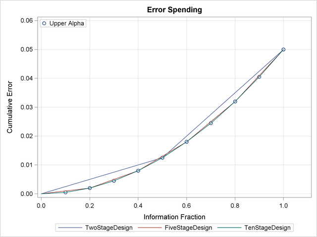
The plot shows similar error spending for these three designs since all three designs are generated from the same power family error spending function.