The PHREG Procedure
- Overview
-
Getting Started

-
Syntax
PROC PHREG Statement ASSESS Statement BASELINE Statement BAYES Statement BY Statement CLASS Statement CONTRAST Statement EFFECT Statement ESTIMATE Statement FREQ Statement HAZARDRATIO Statement ID Statement LSMEANS Statement LSMESTIMATE Statement MODEL Statement OUTPUT Statement Programming Statements RANDOM Statement STRATA Statement SLICE Statement STORE Statement TEST Statement WEIGHT Statement
-
Details
Failure Time Distribution Time and CLASS Variables Usage Partial Likelihood Function for the Cox Model Counting Process Style of Input Left-Truncation of Failure Times The Multiplicative Hazards Model The Frailty Model Hazard Ratios Specifics for Classical Analysis Specifics for Bayesian Analysis Computational Resources Input and Output Data Sets Displayed Output ODS Table Names ODS Graphics
-
Examples
Stepwise Regression Best Subset Selection Modeling with Categorical Predictors Firth’s Correction for Monotone Likelihood Conditional Logistic Regression for m:n Matching Model Using Time-Dependent Explanatory Variables Time-Dependent Repeated Measurements of a Covariate Survivor Function Estimates for Specific Covariate Values Analysis of Residuals Analysis of Recurrent Events Data Analysis of Clustered Data Model Assessment Using Cumulative Sums of Martingale Residuals Bayesian Analysis of the Cox Model Bayesian Analysis of Piecewise Exponential Model
- References
Example 66.8 Survivor Function Estimates for Specific Covariate Values
You might want to use your regression analysis results to generate predicted survival curves for subjects not in the study. The COVARIATES= data set in the BASELINE statement enables you to specify the sets of covariate values for the prediction. By using the PLOTS= option in the PROC PHREG statement, you can display a survival curve for each row of covariates in the COVARIATES= data set. You can elect to output the predicted survival curves in a SAS data set by using just the BASELINE statement. This example illustrates these two tasks by using the Myeloma data in Example 66.1.
In Example 66.1, variables LogBUN and HGB were identified as the most important prognostic factors for the myeloma data. Two sets of covariates for predicting the survivor function are saved in the data set Inrisks in the following DATA step. Also created in this data set is the variable Id, whose values will be used in identifying the covariate sets in the survival plot.
data Inrisks;
   length Id $20;
   input LogBUN HGB Id $12-31;
   datalines;
1.00 10.0  logBUN=1.0 HGB=10
1.80 12.0  logBUN=1.8 HGB=12
;
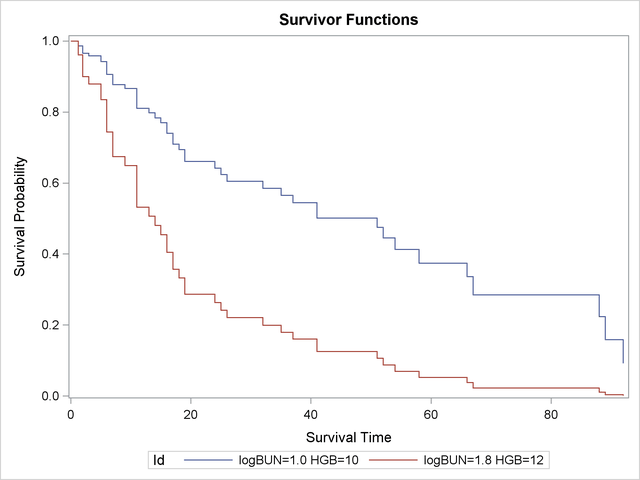
The following statements produce the plot in Output 66.8.1 and create the BASELINE data set Pred1:
ods graphics on;
proc phreg data=Myeloma plots(overlay)=survival;
   model Time*VStatus(0)=LogBUN HGB;
   baseline covariates=Inrisks out=Pred1 survival=_all_ / rowid=Id;
run;
ods graphics off;
The COVARIATES= option in the BASELINE statement specifies the data set that contains the set of covariates of interest. The PLOTS= option in the PROC PHREG statement creates the survivor plot. The OVERLAY suboption overlays the two curves in the same plot. If the OVERLAY suboption is not specified, each curve is displayed in a separate plot. The ROWID= option in the BASELINE statement specifies that the values of the variable Id in the COVARIATES= data set be used to identify the curves in the plot. The SURVIVAL=_ALL_ option in the BASELINE statement requests that the estimated survivor function, standard error, and lower and upper confidence limits for the survivor function be output into the SAS data set specified in the OUT= option.
The survival Plot (Output 66.8.1) contains two curves, one for each of row of covariates in the data set Inrisks.
Finally, PROC PRINT is used to print out the observations in the data set Pred1 for the realization LogBUN=1.00 and HGB=10.0:
proc print data=Pred1(where=(logBUN=1 and HGB=10));
run;
As shown in Output 66.8.2, there are 32 observations representing the survivor function for the realization LogBUN=1.00 and HGB=10.0. The first observation has survival time 0 and survivor function estimate 1.0. Each of the remaining 31 observations represents a distinct event time in the input data set Myeloma. These observations are presented in ascending order of the event times. Note that all the variables in the COVARIATE=InRisks data set are included in the OUT=Pred1 data set. Likewise, you can print out the observations that represent the survivor function for the realization LogBUN=1.80 and HGB=12.0.
| Obs | Id | LogBUN | HGB | Time | Survival | StdErrSurvival | LowerSurvival | UpperSurvival |
|---|---|---|---|---|---|---|---|---|
| 1 | logBUN=1.0 HGB=10 | 1 | 10 | 0.00 | 1.00000 | . | . | . |
| 2 | logBUN=1.0 HGB=10 | 1 | 10 | 1.25 | 0.98678 | 0.01043 | 0.96655 | 1.00000 |
| 3 | logBUN=1.0 HGB=10 | 1 | 10 | 2.00 | 0.96559 | 0.01907 | 0.92892 | 1.00000 |
| 4 | logBUN=1.0 HGB=10 | 1 | 10 | 3.00 | 0.95818 | 0.02180 | 0.91638 | 1.00000 |
| 5 | logBUN=1.0 HGB=10 | 1 | 10 | 5.00 | 0.94188 | 0.02747 | 0.88955 | 0.99729 |
| 6 | logBUN=1.0 HGB=10 | 1 | 10 | 6.00 | 0.90635 | 0.03796 | 0.83492 | 0.98389 |
| 7 | logBUN=1.0 HGB=10 | 1 | 10 | 7.00 | 0.87742 | 0.04535 | 0.79290 | 0.97096 |
| 8 | logBUN=1.0 HGB=10 | 1 | 10 | 9.00 | 0.86646 | 0.04801 | 0.77729 | 0.96585 |
| 9 | logBUN=1.0 HGB=10 | 1 | 10 | 11.00 | 0.81084 | 0.05976 | 0.70178 | 0.93686 |
| 10 | logBUN=1.0 HGB=10 | 1 | 10 | 13.00 | 0.79800 | 0.06238 | 0.68464 | 0.93012 |
| 11 | logBUN=1.0 HGB=10 | 1 | 10 | 14.00 | 0.78384 | 0.06515 | 0.66601 | 0.92251 |
| 12 | logBUN=1.0 HGB=10 | 1 | 10 | 15.00 | 0.76965 | 0.06779 | 0.64762 | 0.91467 |
| 13 | logBUN=1.0 HGB=10 | 1 | 10 | 16.00 | 0.74071 | 0.07269 | 0.61110 | 0.89781 |
| 14 | logBUN=1.0 HGB=10 | 1 | 10 | 17.00 | 0.71005 | 0.07760 | 0.57315 | 0.87966 |
| 15 | logBUN=1.0 HGB=10 | 1 | 10 | 18.00 | 0.69392 | 0.07998 | 0.55360 | 0.86980 |
| 16 | logBUN=1.0 HGB=10 | 1 | 10 | 19.00 | 0.66062 | 0.08442 | 0.51425 | 0.84865 |
| 17 | logBUN=1.0 HGB=10 | 1 | 10 | 24.00 | 0.64210 | 0.08691 | 0.49248 | 0.83717 |
| 18 | logBUN=1.0 HGB=10 | 1 | 10 | 25.00 | 0.62360 | 0.08921 | 0.47112 | 0.82542 |
| 19 | logBUN=1.0 HGB=10 | 1 | 10 | 26.00 | 0.60523 | 0.09136 | 0.45023 | 0.81359 |
| 20 | logBUN=1.0 HGB=10 | 1 | 10 | 32.00 | 0.58549 | 0.09371 | 0.42784 | 0.80122 |
| 21 | logBUN=1.0 HGB=10 | 1 | 10 | 35.00 | 0.56534 | 0.09593 | 0.40539 | 0.78840 |
| 22 | logBUN=1.0 HGB=10 | 1 | 10 | 37.00 | 0.54465 | 0.09816 | 0.38257 | 0.77542 |
| 23 | logBUN=1.0 HGB=10 | 1 | 10 | 41.00 | 0.50178 | 0.10166 | 0.33733 | 0.74639 |
| 24 | logBUN=1.0 HGB=10 | 1 | 10 | 51.00 | 0.47546 | 0.10368 | 0.31009 | 0.72901 |
| 25 | logBUN=1.0 HGB=10 | 1 | 10 | 52.00 | 0.44510 | 0.10522 | 0.28006 | 0.70741 |
| 26 | logBUN=1.0 HGB=10 | 1 | 10 | 54.00 | 0.41266 | 0.10689 | 0.24837 | 0.68560 |
| 27 | logBUN=1.0 HGB=10 | 1 | 10 | 58.00 | 0.37465 | 0.10891 | 0.21192 | 0.66232 |
| 28 | logBUN=1.0 HGB=10 | 1 | 10 | 66.00 | 0.33626 | 0.10980 | 0.17731 | 0.63772 |
| 29 | logBUN=1.0 HGB=10 | 1 | 10 | 67.00 | 0.28529 | 0.11029 | 0.13372 | 0.60864 |
| 30 | logBUN=1.0 HGB=10 | 1 | 10 | 88.00 | 0.22412 | 0.10928 | 0.08619 | 0.58282 |
| 31 | logBUN=1.0 HGB=10 | 1 | 10 | 89.00 | 0.15864 | 0.10317 | 0.04435 | 0.56750 |
| 32 | logBUN=1.0 HGB=10 | 1 | 10 | 92.00 | 0.09180 | 0.08545 | 0.01481 | 0.56907 |