The PHREG Procedure
- Overview
-
Getting Started

-
Syntax
PROC PHREG Statement ASSESS Statement BASELINE Statement BAYES Statement BY Statement CLASS Statement CONTRAST Statement EFFECT Statement ESTIMATE Statement FREQ Statement HAZARDRATIO Statement ID Statement LSMEANS Statement LSMESTIMATE Statement MODEL Statement OUTPUT Statement Programming Statements RANDOM Statement STRATA Statement SLICE Statement STORE Statement TEST Statement WEIGHT Statement
-
Details
Failure Time Distribution Time and CLASS Variables Usage Partial Likelihood Function for the Cox Model Counting Process Style of Input Left-Truncation of Failure Times The Multiplicative Hazards Model The Frailty Model Hazard Ratios Specifics for Classical Analysis Specifics for Bayesian Analysis Computational Resources Input and Output Data Sets Displayed Output ODS Table Names ODS Graphics
-
Examples
Stepwise Regression Best Subset Selection Modeling with Categorical Predictors Firth’s Correction for Monotone Likelihood Conditional Logistic Regression for m:n Matching Model Using Time-Dependent Explanatory Variables Time-Dependent Repeated Measurements of a Covariate Survivor Function Estimates for Specific Covariate Values Analysis of Residuals Analysis of Recurrent Events Data Analysis of Clustered Data Model Assessment Using Cumulative Sums of Martingale Residuals Bayesian Analysis of the Cox Model Bayesian Analysis of Piecewise Exponential Model
- References
| Specifics for Bayesian Analysis |
To request a Bayesian analysis, you specify the new BAYES statement in addition to the PROC PHREG statement and the MODEL statement. You include a CLASS statement if you have effects that involve categorical variables. The FREQ or WEIGHT statement can be included if you have a frequency or weight variable, respectively, in the input data. The STRATA statement can be used to carry out a stratified analysis for the Cox model, but it is not allowed in the piecewise constant baseline hazard model. Programming statements can be used to create time-dependent covariates for the Cox model, but they are not allowed in the piecewise constant baseline hazard model. However, you can use the counting process style of input to accommodate time-dependent covariates that are not continuously changing with time for the piecewise constant baseline hazard model and the Cox model as well. The HAZARDRATIO statement enables you to request a hazard ratio analysis based on the posterior samples. The ASSESS, CONTRAST, ID, OUTPUT, and TEST statements, if specified, are ignored. Also ignored are the COVM and COVS options in the PROC PHREG statement and the following options in the MODEL statement: BEST=, CORRB, COVB, DETAILS, HIERARCHY=, INCLUDE=, MAXSTEP=, NOFIT, PLCONV=, SELECTION=, SEQUENTIAL, SLENTRY=, and SLSTAY=.
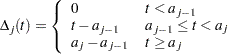
Piecewise Constant Baseline Hazard Model
Single Failure Time Variable
Let  be the observed data. Let
  be a partition of the time axis.
Hazards in Original Scale
The hazard function for subject  is
is
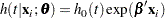 |
where
 |
The baseline cumulative hazard function is
 |
where
 |
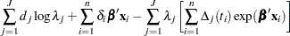
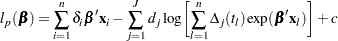
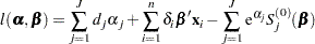
The log likelihood is given by
 |
 |
 |
|||
 |
|
 |
where  .
.
Note that for  , the full conditional for
  is log-concave only when
  , but the full conditionals for the
  ’s are always log-concave.
For a given  ,
,  gives
gives
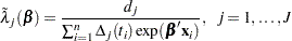 |
Substituting these values into  gives the profile log likelihood for
 |
where 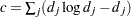 . Since the constant
  does not depend on , it can be discarded from
  in the optimization.
The MLE  of is obtained by maximizing
 |
with respect to , and the MLE  of
of  is given by
 |
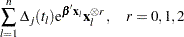
For  , let
, let
 |
|
 |
|||
 |
|
 |
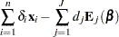
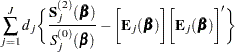
The partial derivatives of are
 |
|
 |
|||
 |
|
 |
The asymptotic covariance matrix for  is obtained as the inverse of the information matrix given by
 |
|
 |
|||
 |
|
 |
|||
 |
|
 |
See Example 6.5.1 in Lawless (2003) for details.
Hazards in Log Scale
By letting
 |
you can build a prior correlation among the ’s by using a correlated prior  , where
 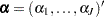 .
.
The log likelihood is given by
 |
Then the MLE of is given by
 |
Note that the full conditionals for  ’s and ’s are always log-concave.
The asymptotic covariance matrix for  is obtained as the inverse of the information matrix formed by
 |
|
 |
|||
 |
|
 |
|||
 |
|
 |
Counting Process Style of Input
Let  be the observed data. Let
  be a partition of the time axis, where
  for all
  .
.
Replacing  with
with
 |
the formulation for the single failure time variable applies.
Priors for Model Parameters
For a Cox model, the model parameters are the regression coefficients. For a piecewise exponential model, the model parameters consist of the regression coefficients and the hazards or log-hazards. The priors for the hazards and the priors for the regression coefficients are assumed to be independent, while you can have a joint multivariate normal prior for the log-hazards and the regression coefficients.
Hazard Parameters
Let  be the constant baseline hazards.
Improper Prior
The joint prior density is given by
 |
This prior is improper (nonintegrable), but the posterior distribution is proper as long as there is at least one event time in each of the constant hazard intervals.
Uniform Prior
The joint prior density is given by
 |
This prior is improper (nonintegrable), but the posteriors are proper as long as there is at least one event time in each of the constant hazard intervals.
Gamma Prior
The gamma distribution  has a pdf
 |
where  is the shape parameter and
  is the scale parameter. The mean is
  and the variance is
  .
.
Independent Gamma Prior
Suppose for , has an independent  prior. The joint prior density is given by
 |
AR1 Prior
 are correlated as follows:
 |
 |
 |
|||
 |
|
 |
|||
 |
|
 |
|||
 |
|
 |
The joint prior density is given by
 |
Log-Hazard Parameters
Write  .
.
Uniform Prior
The joint prior density is given by
 |
Note that the uniform prior for the log-hazards is the same as the improper prior for the hazards.
Normal Prior
Assume  has a multivariate normal prior with mean vector
  and covariance matrix
  . The joint prior density is given by
 |
Regression Coefficients
Let  be the vector of regression coefficients.
Uniform Prior
The joint prior density is given by
 |
This prior is improper, but the posterior distributions for are proper.
Normal Prior
Assume has a multivariate normal prior with mean vector  and covariance matrix
  . The joint prior density is given by
 |
Joint Multivariate Normal Prior for Log-Hazards and Regression Coefficients
Assume  has a multivariate normal prior with mean vector
  and covariance matrix
  . The joint prior density is given by
 |
Zellner’s g-Prior
Assume has a multivariate normal prior with mean vector  and covariance matrix
  , where
  is the design matrix and
  is either a constant or it follows a gamma prior with density
  where and
  are the SHAPE= and ISCALE= parameters. Let
  be the rank of . The joint prior density with g being a constant c is given by
 |
The joint prior density with g having a gamma prior is given by
 |
Posterior Distribution
Denote the observed data by  .
.
Cox Model
 |
where  is the partial likelihood function with regression coefficients as parameters.
Piecewise Exponential Model
Hazard Parameters
 |
where  is the likelihood function with hazards and regression coefficients as parameters.
Log-Hazard Parameters
 |
where  is the likelihood function with log-hazards and regression coefficients as parameters.
Sampling from the Posterior Distribution
For the Gibbs sampler, PROC PHREG uses the ARMS (adaptive rejection Metropolis sampling) algorithm of Gilks, Best, and Tan (1995) to sample from the full conditionals. This is the default sampling scheme. Alternatively, you can requests the random walk Metropolis (RWM) algorithm to sample an entire parameter vector from the posterior distribution. For a general discussion of these algorithms, refer to section Markov Chain Monte Carlo Method.
You can output these posterior samples into a SAS data set by using the OUTPOST= option in the BAYES statement, or you can use the following SAS statement to output the posterior samples into the SAS data set Post:
ods output PosteriorSample=Post;
The output data set also includes the variables LogLike and LogPost, which represent the log of the likelihood and the log of the posterior log density, respectively.
Let  be the parameter vector. For the Cox model, the
  ’s are the regression coefficients
  ’s, and for the piecewise constant baseline hazard model, the ’s consist of the baseline hazards
  ’s (or log baseline hazards
  ’s) and the regression coefficients
  ’s. Let
  be the likelihood function, where is the observed data. Note that for the Cox model, the likelihood contains the infinite-dimensional baseline hazard function, and the gamma process is perhaps the most commonly used prior process (Ibrahim, Chen, and Sinha; 2001). However, Sinha, Ibrahim, and Chen (2003) justify using the partial likelihood as the likelihood function for the Bayesian analysis. Let
  be the prior distribution. The posterior
  is proportional to the joint distribution
  .
.
Gibbs Sampler
The full conditional distribution of is proportional to the joint distribution; that is,
 |
For example, the one-dimensional conditional distribution of  , given
  , is computed as
 |
Suppose you have a set of arbitrary starting values  . Using the ARMS algorithm, an iteration of the Gibbs sampler consists of the following:
draw
 from
from 
draw
 from
from 

draw
 from
from 
After one iteration, you have  . After
  iterations, you have
  . Cumulatively, a chain of samples is obtained.
Random Walk Metropolis Algorithm
PROC PHREG uses a multivariate normal proposal distribution  centered at
  . With an initial parameter vector
  , a new sample
  is obtained as follows:
sample
 from
from 
calculate the quantity

sample
 from the uniform distribution
set
 if
if  ; otherwise set
With taking the role of , the previous steps are repeated to generate the next sample  . After iterations, a chain of samples
  is obtained.
Starting Values of the Markov Chains
When the BAYES statement is specified, PROC PHREG generates one Markov chain that contains the approximate posterior samples of the model parameters. Additional chains are produced when the Gelman-Rubin diagnostics are requested. Starting values (initial values) can be specified in the INITIAL= data set in the BAYES statement. If the INITIAL= option is not specified, PROC PHREG picks its own initial values for the chains based on the maximum likelihood estimates of and the prior information of .
Denote  as the integral value of
  .
.
Constant Baseline Hazards ’s
For the first chain that the summary statistics and diagnostics are based on, the initial values are
 |
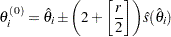
For subsequent chains, the starting values are picked in two different ways according to the total number of chains specified. If the total number of chains specified is less than or equal to 10, initial values of the  th chain (
 ) are given by
 |
with the plus sign for odd and minus sign for even . If the total number of chains is greater than 10, initial values are picked at random over a wide range of values. Let  be a uniform random number between 0 and 1; the initial value for is given by
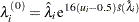 |
Regression Coefficients and Log-Hazard Parameters ’s
The ’s are the regression coefficients ’s, and in the piecewise exponential model, include the log-hazard parameters ’s. For the first chain that the summary statistics and regression diagnostics are based on, the initial values are
 |
If the number of chains requested is less than or equal to 10, initial values for the th chain ( ) are given by
 |
with the plus sign for odd and minus sign for even . When there are more than 10 chains, the initial value for the is picked at random over the range  ; that is,
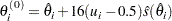 |
where is a uniform random number between 0 and 1.
Fit Statistics
Denote the observed data by . Let be the vector of parameters of length . Let be the likelihood. The deviance information criterion (DIC) proposed in Spiegelhalter et al. (2002) is a Bayesian model assessment tool. Let Dev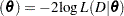 . Let
. Let  and
and  be the corresponding posterior means of
  and , respectively. The deviance information criterion is computed as
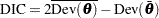 |
Also computed is
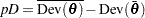 |
where  is interpreted as the effective number of parameters.
Note that defined here does not have the standardizing term as in the section Deviance Information Criterion (DIC). Nevertheless, the DIC calculated here is still useful for variable selection.
Posterior Distribution for Quantities of Interest
Let be the parameter vector. For the Cox model, the ’s are the regression coefficients ’s; for the piecewise constant baseline hazard model, the ’s consist of the baseline hazards ’s (or log baseline hazards ’s) and the regression coefficients ’s. Let  be the chain that represents the posterior distribution for .
Consider a quantity of interest  that can be expressed as a function
  of the parameter vector . You can construct the posterior distribution of by evaluating the function
  for each
  in
in  . The posterior chain for is
  Summary statistics such as mean, standard deviation, percentiles, and credible intervals are used to describe the posterior distribution of .
Hazard Ratio
As shown in the section Hazard Ratios, a log-hazard ratio is a linear combination of the regression coefficients. Let  be the vector of linear coefficients. The posterior sample for this hazard ratio is the set
  .
.
Survival Distribution
Let  be a covariate vector of interest.
Cox Model
Let  be the observed data. Define
 |
Consider the th draw  of . The baseline cumulative hazard function at time
  is given by
 |
For the given covariate vector , the cumulative hazard function at time is
 |
and the survival function at time is
 |
Piecewise Exponential Model
Let  be a partition of the time axis. Consider the th draw in , where consists of
  and . The baseline cumulative hazard function at time is
 |
where
|
For the given covariate vector  , the cumulative hazard function at time is
 |
and the survival function at time is
 |