The LOGISTIC Procedure
- Overview
- Getting Started
-
Syntax
 PROC LOGISTIC Statement BY Statement CLASS Statement CONTRAST Statement EFFECT Statement EFFECTPLOT Statement ESTIMATE Statement EXACT Statement EXACTOPTIONS Statement FREQ Statement LSMEANS Statement LSMESTIMATE Statement MODEL Statement ODDSRATIO Statement OUTPUT Statement ROC Statement ROCCONTRAST Statement SCORE Statement SLICE Statement STORE Statement STRATA Statement TEST Statement UNITS Statement WEIGHT Statement
 -
Details
Missing Values Response Level Ordering Link Functions and the Corresponding Distributions Determining Observations for Likelihood Contributions Iterative Algorithms for Model Fitting Convergence Criteria Existence of Maximum Likelihood Estimates Effect-Selection Methods Model Fitting Information Generalized Coefficient of Determination Score Statistics and Tests Confidence Intervals for Parameters Odds Ratio Estimation Rank Correlation of Observed Responses and Predicted Probabilities Linear Predictor, Predicted Probability, and Confidence Limits Classification Table Overdispersion The Hosmer-Lemeshow Goodness-of-Fit Test Receiver Operating Characteristic Curves Testing Linear Hypotheses about the Regression Coefficients Regression Diagnostics Scoring Data Sets Conditional Logistic Regression Exact Conditional Logistic Regression Input and Output Data Sets Computational Resources Displayed Output ODS Table Names ODS Graphics
-
Examples
Stepwise Logistic Regression and Predicted Values Logistic Modeling with Categorical Predictors Ordinal Logistic Regression Nominal Response Data: Generalized Logits Model Stratified Sampling Logistic Regression Diagnostics ROC Curve, Customized Odds Ratios, Goodness-of-Fit Statistics, R-Square, and Confidence Limits Comparing Receiver Operating Characteristic Curves Goodness-of-Fit Tests and Subpopulations Overdispersion Conditional Logistic Regression for Matched Pairs Data Firth’s Penalized Likelihood Compared with Other Approaches Complementary Log-Log Model for Infection Rates Complementary Log-Log Model for Interval-Censored Survival Times Scoring Data Sets Using the LSMEANS Statement
- References
| Scoring Data Sets |
Scoring a data set, which is especially important for predictive modeling, means applying a previously fitted model to a new data set in order to compute the conditional, or posterior, probabilities of each response category given the values of the explanatory variables in each observation.
The SCORE statement enables you to score new data sets and output the scored values and, optionally, the corresponding confidence limits into a SAS data set. If the response variable is included in the new data set, then you can request fit statistics for the data, which is especially useful for test or validation data. If the response is binary, you can also create a SAS data set containing the receiver operating characteristic (ROC) curve. You can specify multiple SCORE statements in the same invocation of PROC LOGISTIC.
By default, the posterior probabilities are based on implicit prior probabilities that are proportional to the frequencies of the response categories in the training data (the data used to fit the model). Explicit prior probabilities should be specified with the PRIOR= or PRIOREVENT= option when the sample proportions of the response categories in the training data differ substantially from the operational data to be scored. For example, to detect a rare category, it is common practice to use a training set in which the rare categories are overrepresented; without prior probabilities that reflect the true incidence rate, the predicted posterior probabilities for the rare category will be too high. By specifying the correct priors, the posterior probabilities are adjusted appropriately.
The model fit to the DATA= data set in the PROC LOGISTIC statement is the default model used for the scoring. Alternatively, you can save a model fit in one run of PROC LOGISTIC and use it to score new data in a subsequent run. The OUTMODEL= option in the PROC LOGISTIC statement saves the model information in a SAS data set. Specifying this data set in the INMODEL= option of a new PROC LOGISTIC run will score the DATA= data set in the SCORE statement without refitting the model.
The STORE statement can also be used to save your model. The PLM procedure can use this model to score new data sets; see Chapter 68, The PLM Procedure, for more information. You cannot specify priors in PROC PLM.
Fit Statistics for Scored Data Sets
Specifying the FITSTAT option displays the following fit statistics when the data set being scored includes the response variable:
Statistic |
Description |
|---|---|
Total frequency |
|
Total weight |
|
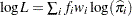
Log likelihood |
|
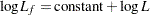
Full log likelihood |
|
Misclassification (error) rate |
|
AIC |
|
AICC |
|
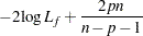
BIC |
|
SC |
|
R-square |
|
Maximum-rescaled R-square |
|
AUC |
Area under the ROC curve |
Brier score (polytomous response) |
|
Brier score (binary response) |
|
Brier reliability (events/trials syntax) |
|


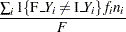


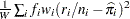
In the preceding table,  is the frequency of the
  th observation in the data set being scored,
  is the weight of the observation, and
  . The number of trials when events/trials syntax is specified is
  , and with single-trial syntax
  . The values
  and
and  are described in the section OUT= Output Data Set in a SCORE Statement. The indicator function
  is
is  if
if  is true and
  otherwise. The likelihood of the model is
  , and
, and  denotes the likelihood of the intercept-only model. For polytomous response models,
  is the observed polytomous response level,
  is the predicted probability of the
  th response level for observation , and
  . For binary response models,
  is the predicted probability of the observation,
  is the number of events when you specify events/trials syntax, and
  when you specify single-trial syntax.
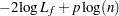
The log likelihood, Akaike’s information criterion (AIC), and Schwarz criterion (SC) are described in the section Model Fitting Information. The full log likelihood is displayed for models specified with events/trials syntax, and the constant term is described in the section Model Fitting Information. The AICC is a small-sample bias-corrected version of the AIC (Hurvich and Tsai; 1993; Burnham and Anderson; 1998). The Bayesian information criterion (BIC) is the same as the SC except when events/trials syntax is specified. The area under the ROC curve for binary response models is defined in the section ROC Computations. The R-square and maximum-rescaled R-square statistics, defined in Generalized Coefficient of Determination, are not computed when you specify both an OFFSET= variable and the INMODEL= data set. The Brier score (Brier; 1950) is the weighted squared difference between the predicted probabilities and their observed response levels. For events/trials syntax, the Brier reliability is the weighted squared difference between the predicted probabilities and the observed proportions (Murphy; 1973).
Posterior Probabilities and Confidence Limits
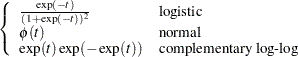
Let  be the inverse link function. That is,
 |
 |
The first derivative of is given by
 |
 |
Suppose there are  response categories. Let Y be the response variable with levels
  . Let
. Let  be a
be a  -vector of covariates, with
  . Let
. Let  be the vector of intercept and slope regression parameters.
Posterior probabilities are given by
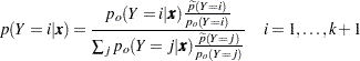 |
where the old posterior probabilities ( ) are the conditional probabilities of the response categories given
  , the old priors (
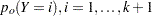 ) are the sample proportions of response categories of the training data, and the new priors (
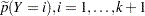 ) are specified in the PRIOR= or PRIOREVENT= option. To simplify notation, absorb the old priors into the new priors; that is
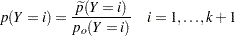 |
Note if the PRIOR= and PRIOREVENT= options are not specified, then  .
.
The posterior probabilities are functions of and their estimates are obtained by substituting by its MLE  . The variances of the estimated posterior probabilities are given by the delta method as follows:
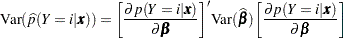 |
where
 |
and the old posterior probabilities  are described in the following sections.
A 100( )% confidence interval for
  is
is
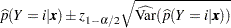 |
where  is the upper 100
 percentile of the standard normal distribution.
Binary and Cumulative Response Models
Let  be the intercept parameters and let
  be the vector of slope parameters. Denote
  . Let
. Let
 |
Estimates of  are obtained by substituting the maximum likelihood estimate for .
The predicted probabilities of the responses are
 |
For  , let
, let  be a () column vector with th entry equal to 1, th entry equal to , and all other entries 0. The derivative of with respect to are
 |
 |
The cumulative posterior probabilities are
 |
Their derivatives are
 |
In the delta-method equation for the variance, replace  with
with  .
.
Finally, for the cumulative response model, use
 |
 |
 |
|||
 |
|
 |
|||
 |
|
 |
|||
 |
|
 |
Generalized Logit Model
Consider the last response level (Y=k+1) as the reference. Let  be the (intercept and slope) parameter vectors for the first
  logits, respectively. Denote
  . Let
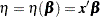
. Let  with
with
 |
Estimates of are obtained by substituting the maximum likelihood estimate for .
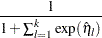
The predicted probabilities are
 |
 |
 |
|||
 |
|
 |
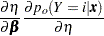
The derivative of with respect to are
 |
|
 |
|||
 |
 |
 |
where
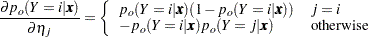 |
Special Case of Binary Response Model with No Priors
Let be the vector of regression parameters. Let
 |
The variance of  is given by
 |
A 100() percent confidence interval for  is
is
 |
Estimates of  and confidence intervals for the are obtained by back-transforming and the confidence intervals for , respectively. That is,
 |
and the confidence intervals are
 |