| The LOGISTIC Procedure |
Example 51.4 Nominal Response Data: Generalized Logits Model
Over the course of one school year, third graders from three different schools are exposed to three different styles of mathematics instruction: a self-paced computer-learning style, a team approach, and a traditional class approach. The students are asked which style they prefer and their responses, classified by the type of program they are in (a regular school day versus a regular day supplemented with an afternoon school program), are displayed in Table 51.13. The data set is from Stokes, Davis, and Koch (2000), and is also analyzed in the section Generalized Logits Model of Chapter 28, The CATMOD Procedure.
Learning Style Preference |
||||
|---|---|---|---|---|
School |
Program |
Self |
Team |
Class |
1 |
Regular |
10 |
17 |
26 |
1 |
Afternoon |
5 |
12 |
50 |
2 |
Regular |
21 |
17 |
26 |
2 |
Afternoon |
16 |
12 |
36 |
3 |
Regular |
15 |
15 |
16 |
3 |
Afternoon |
12 |
12 |
20 |
The levels of the response variable (self, team, and class) have no essential ordering, so a logistic regression is performed on the generalized logits. The model to be fit is
 |
where  is the probability that a student in school
  and program
  prefers teaching style
  ,
,  , and style
  is the baseline style (in this case, class). There are separate sets of intercept parameters
  and regression parameters
  for each logit, and the vector
  is the set of explanatory variables for the
  th population. Thus, two logits are modeled for each school and program combination: the logit comparing self to class and the logit comparing team to class.
The following statements create the data set school and request the analysis. The LINK=GLOGIT option forms the generalized logits. The response variable option ORDER=DATA means that the response variable levels are ordered as they exist in the data set: self, team, and class; thus, the logits are formed by comparing self to class and by comparing team to class. The ODDSRATIO statement produces odds ratios in the presence of interactions, and the ODS GRAPHICS ON statement produces a graphical display of the requested odds ratios.
data school;
   length Program $ 9;
   input School Program $ Style $ Count @@;
   datalines;
1 regular   self 10  1 regular   team 17  1 regular   class 26
1 afternoon self  5  1 afternoon team 12  1 afternoon class 50
2 regular   self 21  2 regular   team 17  2 regular   class 26
2 afternoon self 16  2 afternoon team 12  2 afternoon class 36
3 regular   self 15  3 regular   team 15  3 regular   class 16
3 afternoon self 12  3 afternoon team 12  3 afternoon class 20
;
ods graphics on;
proc logistic data=school;
   freq Count;
   class School Program(ref=first);
   model Style(order=data)=School Program School*Program / link=glogit;
   oddsratio program;
run;
ods graphics off;
Summary information about the model, the response variable, and the classification variables are displayed in Output 51.4.1.
| Model Information | |
|---|---|
| Data Set | WORK.SCHOOL |
| Response Variable | Style |
| Number of Response Levels | 3 |
| Frequency Variable | Count |
| Model | generalized logit |
| Optimization Technique | Newton-Raphson |
| Number of Observations Read | 18 |
|---|---|
| Number of Observations Used | 18 |
| Sum of Frequencies Read | 338 |
| Sum of Frequencies Used | 338 |
| Response Profile | ||
|---|---|---|
| Ordered Value |
Style | Total Frequency |
| 1 | self | 79 |
| 2 | team | 85 |
| 3 | class | 174 |
The "Testing Global Null Hypothesis: BETA=0" table in Output 51.4.2 shows that the parameters are significantly different from zero.
However, the "Type 3 Analysis of Effects" table in Output 51.4.3 shows that the interaction effect is clearly nonsignificant.
| Type 3 Analysis of Effects | |||
|---|---|---|---|
| Effect | DF | Wald Chi-Square |
Pr > ChiSq |
| School | 4 | 14.5522 | 0.0057 |
| Program | 2 | 10.4815 | 0.0053 |
| School*Program | 4 | 1.7439 | 0.7827 |
| Analysis of Maximum Likelihood Estimates | ||||||||
|---|---|---|---|---|---|---|---|---|
| Parameter | Style | DF | Estimate | Standard Error |
Wald Chi-Square |
Pr > ChiSq | ||
| Intercept | self | 1 | -0.8097 | 0.1488 | 29.5989 | <.0001 | ||
| Intercept | team | 1 | -0.6585 | 0.1366 | 23.2449 | <.0001 | ||
| School | 1 | self | 1 | -0.8194 | 0.2281 | 12.9066 | 0.0003 | |
| School | 1 | team | 1 | -0.2675 | 0.1881 | 2.0233 | 0.1549 | |
| School | 2 | self | 1 | 0.2974 | 0.1919 | 2.4007 | 0.1213 | |
| School | 2 | team | 1 | -0.1033 | 0.1898 | 0.2961 | 0.5863 | |
| Program | regular | self | 1 | 0.3985 | 0.1488 | 7.1684 | 0.0074 | |
| Program | regular | team | 1 | 0.3537 | 0.1366 | 6.7071 | 0.0096 | |
| School*Program | 1 | regular | self | 1 | 0.2751 | 0.2281 | 1.4547 | 0.2278 |
| School*Program | 1 | regular | team | 1 | 0.1474 | 0.1881 | 0.6143 | 0.4332 |
| School*Program | 2 | regular | self | 1 | -0.0998 | 0.1919 | 0.2702 | 0.6032 |
| School*Program | 2 | regular | team | 1 | -0.0168 | 0.1898 | 0.0079 | 0.9293 |
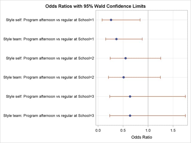
The table produced by the ODDSRATIO statement is displayed in Output 51.4.4. The differences between the program preferences are small across all the styles (logits) compared to their variability as displayed by the confidence limits in Output 51.4.5, confirming that the interaction effect is nonsignificant.
| Wald Confidence Interval for Odds Ratios | |||
|---|---|---|---|
| Label | Estimate | 95% Confidence Limits | |
| Style self: Program afternoon vs regular at School=1 | 0.260 | 0.080 | 0.841 |
| Style team: Program afternoon vs regular at School=1 | 0.367 | 0.153 | 0.883 |
| Style self: Program afternoon vs regular at School=2 | 0.550 | 0.242 | 1.253 |
| Style team: Program afternoon vs regular at School=2 | 0.510 | 0.208 | 1.247 |
| Style self: Program afternoon vs regular at School=3 | 0.640 | 0.234 | 1.747 |
| Style team: Program afternoon vs regular at School=3 | 0.640 | 0.234 | 1.747 |
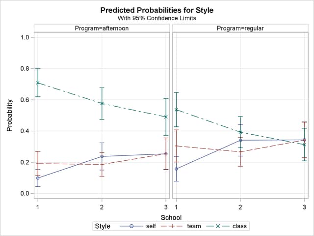
Since the interaction effect is clearly nonsignificant, a main-effects model is fit with the following statements. The EFFECTPLOT statement creates a plot of the predicted values versus the levels of the School variable at each level of the Program variables. The CLM option adds confidence bars, and the NOOBS option suppresses the display of the observations.
ods graphics on;
proc logistic data=school;
   freq Count;
   class School Program(ref=first);
   model Style(order=data)=School Program / link=glogit;
   effectplot interaction(plotby=Program) / clm noobs;
run;
ods graphics off;
All of the global fit tests in Output 51.4.6 suggest the model is significant, and the Type 3 tests show that the school and program effects are also significant.
The parameter estimates, tests for individual parameters, and odds ratios are displayed in Output 51.4.7. The Program variable has nearly the same effect on both logits, while School=1 has the largest effect of the schools.
| Analysis of Maximum Likelihood Estimates | |||||||
|---|---|---|---|---|---|---|---|
| Parameter | Style | DF | Estimate | Standard Error |
Wald Chi-Square |
Pr > ChiSq | |
| Intercept | self | 1 | -0.7978 | 0.1465 | 29.6502 | <.0001 | |
| Intercept | team | 1 | -0.6589 | 0.1367 | 23.2300 | <.0001 | |
| School | 1 | self | 1 | -0.7992 | 0.2198 | 13.2241 | 0.0003 |
| School | 1 | team | 1 | -0.2786 | 0.1867 | 2.2269 | 0.1356 |
| School | 2 | self | 1 | 0.2836 | 0.1899 | 2.2316 | 0.1352 |
| School | 2 | team | 1 | -0.0985 | 0.1892 | 0.2708 | 0.6028 |
| Program | regular | self | 1 | 0.3737 | 0.1410 | 7.0272 | 0.0080 |
| Program | regular | team | 1 | 0.3713 | 0.1353 | 7.5332 | 0.0061 |
| Odds Ratio Estimates | ||||
|---|---|---|---|---|
| Effect | Style | Point Estimate | 95% Wald Confidence Limits |
|
| School 1 vs 3 | self | 0.269 | 0.127 | 0.570 |
| School 1 vs 3 | team | 0.519 | 0.267 | 1.010 |
| School 2 vs 3 | self | 0.793 | 0.413 | 1.522 |
| School 2 vs 3 | team | 0.622 | 0.317 | 1.219 |
| Program regular vs afternoon | self | 2.112 | 1.215 | 3.670 |
| Program regular vs afternoon | team | 2.101 | 1.237 | 3.571 |
The interaction plots in Output 51.4.8 show that School=1 and Program=afternoon have a preference for the traditional classroom style. Of course, since these are not simultaneous confidence intervals, the nonoverlapping 95% confidence limits do not take the place of an actual test.
Copyright © SAS Institute, Inc. All Rights Reserved.