| The NLPC Nonlinear Optimization Solver |
Example 12.1 Least Squares Problem
Although the current release of the NLPC solver does not implement techniques specialized for least squares problems, this example illustrates how the NLPC solver can solve least squares problems by using general nonlinear optimization techniques. The following Bard function (see Moré, Garbow, and Hillstrom; 1981) is a least squares problem with  parameters and
  residual functions
  :
:
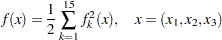 |
where
 |
with  ,
,  ,
, 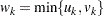 , and
, and
 |
The minimum function value  E–3 is at the point
 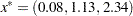 . The starting point
  is used.
You can use the following SAS code to formulate and solve this least squares problem:
proc optmodel;
   set S = 1..15;
   number u{k in S} = k;
   number v{k in S} = 16 - k;
   number w{k in S} = min(u[k], v[k]);
   number y{S} = [ .14 .18 .22 .25 .29 .32 .35 .39 .37 .58
                   .73 .96 1.34 2.10 4.39 ];
   var x{1..3} init 1;

   min f = 0.5*sum{k in S} ( y[k] -
             ( x[1] + u[k]/(v[k]*x[2] + w[k]*x[3]) )
           )^2;
   solve with nlpc / printfreq=1;
   print x;
quit;
A problem summary is displayed in Output 12.1.1. Since there is no explicit optimization technique specified (using the TECH= option), the default algorithm of the trust region method is used. Output 12.1.2 displays the iteration log. The solution summary and the solution are shown in Output 12.1.3.
| Iteration Log: Trust Region Method | ||||
|---|---|---|---|---|
| Iter | Function Calls |
Objective Value |
Optimality Error |
Trust Region Radius |
| 0 | 0 | 20.8408 | 1.2445 | . |
| 1 | 1 | 2.8333 | 2.7031 | 1.000 |
| 2 | 2 | 0.6302 | 2.3180 | 0.989 |
| 3 | 3 | 0.1077 | 0.7732 | 0.998 |
| 4 | 4 | 0.009011 | 0.1396 | 1.007 |
| 5 | 5 | 0.004134 | 0.0125 | 1.042 |
| 6 | 6 | 0.004107 | 0.0000805 | 0.199 |
| 7 | 7 | 0.004107 | 4.3523E-8 | 0.0207 |
| Note: | Optimality criteria (ABSOPTTOL=0.001, OPTTOL=1E-6) are satisfied. |
Alternatively, you can specify the Newton-type method with line search by using the following statement:
solve with nlpc / tech=newtyp printfreq=1;
You get the output for the NEWTYP method as shown in Output 12.1.4 and Output 12.1.5.
| Iteration Log: Newton-Type Method with Line Search | |||||
|---|---|---|---|---|---|
| Iter | Function Calls |
Objective Value |
Optimality Error |
Step Size |
Slope of Search Direction |
| 0 | 0 | 20.8408 | 1.2445 | . | . |
| 1 | 1 | 2.2590 | 2.6880 | 1.000 | -35.485 |
| 2 | 2 | 0.6235 | 2.3158 | 1.000 | -2.577 |
| 3 | 3 | 0.1116 | 0.7488 | 1.000 | -0.831 |
| 4 | 4 | 0.0115 | 0.1703 | 1.000 | -0.172 |
| 5 | 5 | 0.004188 | 0.0167 | 1.000 | -0.0136 |
| 6 | 6 | 0.004109 | 0.000427 | 1.000 | -0.0002 |
| 7 | 7 | 0.004109 | 0.0000637 | 1.000 | -578E-9 |
| 8 | 8 | 0.004108 | 0.0000352 | 1.000 | -95E-8 |
| 9 | 9 | 0.004107 | 8.7568E-6 | 1.000 | -52E-8 |
| 10 | 10 | 0.004107 | 1.1411E-6 | 1.000 | -33E-9 |
| 11 | 11 | 0.004107 | 8.2006E-8 | 1.000 | -63E-11 |
| Note: | Optimality criteria (ABSOPTTOL=0.001, OPTTOL=1E-6) are satisfied. |
You can also select the conjugate gradient method as follows:
solve with nlpc / tech=congra printfreq=2;
Note that the PRINTFREQ= option was used to reduce the number of rows in the iteration log. As Output 12.1.6 shows, only every other iteration is displayed. Output 12.1.7 gives a summary of the solution and prints the solution.
| Iteration Log: Conjugate Gradient Method | ||||||
|---|---|---|---|---|---|---|
| Iter | Function Calls |
Objective Value |
Optimality Error |
Step Size |
Slope of Search Direction |
Restarts |
| 0 | 0 | 20.8408 | 1.2445 | . | . | 0 |
| 2 | 4 | 0.7199 | 1.1503 | 0.108 | -11.045 | 1 |
| 4 | 10 | 0.0119 | 0.4362 | 0.150 | -0.0010 | 2 |
| 6 | 14 | 0.004903 | 0.008169 | 35.849 | -0.0001 | 3 |
| 8 | 19 | 0.004788 | 0.0819 | 22.628 | -0.0001 | 4 |
| 10 | 24 | 0.004233 | 0.0436 | 0.679 | -0.0034 | 6 |
| 12 | 28 | 0.004201 | 0.0191 | 0.345 | -0.0001 | 7 |
| 14 | 32 | 0.004166 | 0.0161 | 20.000 | -129E-7 | 8 |
| 16 | 36 | 0.004160 | 0.003508 | 0.112 | -205E-8 | 9 |
| 18 | 40 | 0.004108 | 0.001920 | 9.125 | -108E-7 | 10 |
| 20 | 44 | 0.004108 | 0.000637 | 2.000 | -178E-9 | 12 |
| 22 | 48 | 0.004107 | 0.000581 | 0.291 | -245E-9 | 13 |
| 24 | 52 | 0.004107 | 2.5337E-6 | 2.000 | -62E-13 | 14 |
| 25 | 54 | 0.004107 | 7.4262E-8 | 0.142 | -15E-12 | 14 |
| Note: | Optimality criteria (ABSOPTTOL=0.001, OPTTOL=1E-6) are satisfied. |
Although the number of iterations required for each optimization technique to converge varies, all three techniques produce the identical solution, given the same starting point.
Copyright © SAS Institute, Inc. All Rights Reserved.