The X13 Procedure
- Overview
-
Getting Started

-
SyntaxFunctional SummaryPROC X13 StatementADJUST StatementARIMA StatementAUTOMDL StatementBY StatementCHECK StatementESTIMATE StatementEVENT StatementFORECAST StatementID StatementIDENTIFY StatementINPUT StatementOUTLIER StatementOUTPUT StatementPICKMDL StatementREGRESSION StatementSEATSDECOMP StatementTABLES StatementTRANSFORM StatementUSERDEFINED StatementVAR StatementX11 Statement
-
DetailsData RequirementsMissing ValuesSAS Predefined EventsUser-Defined Regression VariablesCombined Test for the Presence of Identifiable SeasonalityComputationsPICKMDL Model SelectionSEATS DecompositionDisplayed Output, ODS Table Names, and OUTPUT Tablename KeywordsTable D 8.BUsing Auxiliary Variables to Subset Output Data SetsODS GraphicsOUT= Data SetSEATSDECOMP OUT= Data SetSpecial Data Sets
-
ExamplesARIMA Model IdentificationModel EstimationSeasonal AdjustmentRegARIMA Automatic Model SelectionAutomatic Outlier DetectionUser-Defined RegressorsMDLINFOIN= and MDLINFOOUT= Data SetsSetting Regression ParametersCreating an MDLINFO= Data Set for Use with the PICKMDL StatementIllustration of ODS GraphicsAUXDATA= Data Set
- References
Basic Seasonal Adjustment
Suppose that you have monthly retail sales data starting in September 1978 in a SAS data set named SALES. At this point, you do not suspect that any calendar effects are present, and there are no prior adjustments that need to
be made to the data.
In this simplest case, you need only specify the DATE= variable in the PROC X13 statement and request seasonal adjustment in the X11 statement as shown in the following statements:
data sales;
   set sashelp.air;
   sales = air;
   date = intnx( 'month', '01sep78'd, _n_-1 );
   format date monyy.;
run;
proc x13 data=sales date=date;
   var sales;
   x11;
   ods select d11;
run;
The results of the seasonal adjustment are in Table D11 (the final seasonally adjusted series) in the displayed output shown in Figure 45.1.
Figure 45.1: Basic Seasonal Adjustment
| Table D 11: Final Seasonally Adjusted Data For Variable sales |
|||||||||||||
|---|---|---|---|---|---|---|---|---|---|---|---|---|---|
| Year | JAN | FEB | MAR | APR | MAY | JUN | JUL | AUG | SEP | OCT | NOV | DEC | Total |
| 1978 | . | . | . | . | . | . | . | . | 124.560 | 124.649 | 124.920 | 129.002 | 503.131 |
| 1979 | 125.087 | 126.759 | 125.252 | 126.415 | 127.012 | 130.041 | 128.056 | 129.165 | 127.182 | 133.847 | 133.199 | 135.847 | 1547.86 |
| 1980 | 128.767 | 139.839 | 143.883 | 144.576 | 148.048 | 145.170 | 140.021 | 153.322 | 159.128 | 161.614 | 167.996 | 165.388 | 1797.75 |
| 1981 | 175.984 | 166.805 | 168.380 | 167.913 | 173.429 | 175.711 | 179.012 | 182.017 | 186.737 | 197.367 | 183.443 | 184.907 | 2141.71 |
| 1982 | 186.080 | 203.099 | 193.386 | 201.988 | 198.322 | 205.983 | 210.898 | 213.516 | 213.897 | 218.902 | 227.172 | 240.453 | 2513.69 |
| 1983 | 231.839 | 224.165 | 219.411 | 225.907 | 225.015 | 226.535 | 221.680 | 222.177 | 222.959 | 212.531 | 230.552 | 232.565 | 2695.33 |
| 1984 | 237.477 | 239.870 | 246.835 | 242.642 | 244.982 | 246.732 | 251.023 | 254.210 | 264.670 | 266.120 | 266.217 | 276.251 | 3037.03 |
| 1985 | 275.485 | 281.826 | 294.144 | 286.114 | 293.192 | 296.601 | 293.861 | 309.102 | 311.275 | 319.239 | 319.936 | 323.663 | 3604.44 |
| 1986 | 326.693 | 330.341 | 330.383 | 330.792 | 333.037 | 332.134 | 336.444 | 341.017 | 346.256 | 350.609 | 361.283 | 362.519 | 4081.51 |
| 1987 | 364.951 | 371.274 | 369.238 | 377.242 | 379.413 | 376.451 | 378.930 | 375.392 | 374.940 | 373.612 | 368.753 | 364.885 | 4475.08 |
| 1988 | 371.618 | 383.842 | 385.849 | 404.810 | 381.270 | 388.689 | 385.661 | 377.706 | 397.438 | 404.247 | 414.084 | 416.486 | 4711.70 |
| 1989 | 426.716 | 419.491 | 427.869 | 446.161 | 438.317 | 440.639 | 450.193 | 454.638 | 460.644 | 463.209 | 427.728 | 485.386 | 5340.99 |
| 1990 | 477.259 | 477.753 | 483.841 | 483.056 | 481.902 | 499.200 | 484.893 | 485.245 | . | . | . | . | 3873.15 |
| Avg | 277.330 | 280.422 | 282.373 | 286.468 | 285.328 | 288.657 | 288.389 | 291.459 | 265.807 | 268.829 | 268.774 | 276.446 | |
| Total: 40323 Mean: 280.02 S.D.: 111.31 Min: 124.56 Max: 499.2 |
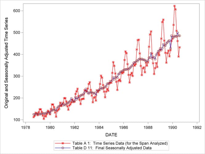
You can compare the original series (Table A1) and the final seasonally adjusted series (Table D11) by plotting them together as shown in Figure 45.2. These tables are requested in the OUTPUT statement and are written to the OUT= data set. Note that the default variable name used in the output data set is the input variable name followed by an underscore and the corresponding table name.
proc x13 data=sales date=date noprint;
   var sales;
   x11;
   output out=out a1 d11;
run;

proc sgplot data=out;
   series x=date y=sales_A1 / name = "A1" markers
                              markerattrs=(color=red symbol='asterisk')
                              lineattrs=(color=red);
   series x=date y=sales_D11 / name= "D11" markers
                               markerattrs=(symbol='circle')
                               lineattrs=(color=blue);
   yaxis label='Original and Seasonally Adjusted Time Series';
run;
Figure 45.2: Plot of Original and Seasonally Adjusted Data