The X13 Procedure

Example 45.1 ARIMA Model Identification

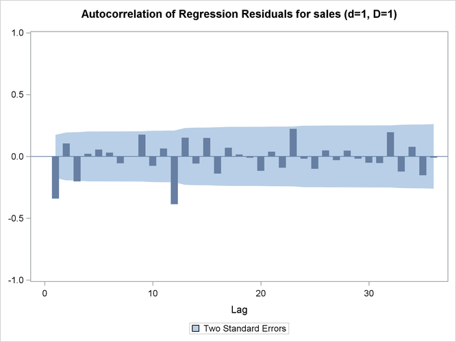
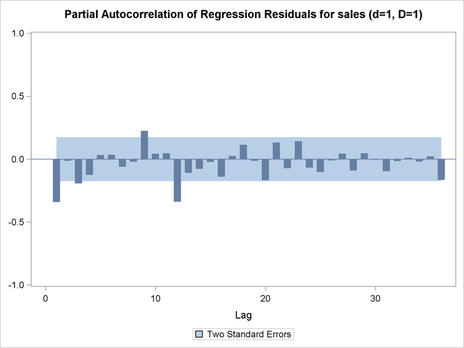
This example shows typical PROC X13 statements that are used for ARIMA model identification. This example invokes the X13 procedure and uses the TRANSFORM and IDENTIFY statements. It specifies the time series data, takes the logarithm of the series (TRANSFORM statement), and generates ACFs and PACFs for the specified levels of differencing (IDENTIFY statement). The ACFs and PACFs for DIFF=1 and SDIFF=1 are shown in Output 45.1.1, Output 45.1.2, Output 45.1.3, and Output 45.1.4. The data set is the same as in the section Basic Seasonal Adjustment.

The graphical displays are available when ODS Graphics is enabled. For more information about the graphics available in the X13 procedure, see the section ODS Graphics.

proc x13 data=sales date=date;
   var sales;
   transform power=0;
   identify diff=(0,1) sdiff=(0,1);
run;

Output 45.1.1: ACFs (Nonseasonal Order=1 Seasonal Order=1)

The X13 Procedure

Autocorrelation of Regression Residuals for ARIMA Model Identification
For Variable sales
Differencing: Nonseasonal Order=1 Seasonal Order=1

Lag	Correlation	Standard Error	Chi-Square	DF	Pr > ChiSq
1	-0.34112	0.08737	15.5957	1	<.0001
2	0.10505	0.09701	17.0860	2	0.0002
3	-0.20214	0.09787	22.6478	3	<.0001
4	0.02136	0.10101	22.7104	4	0.0001
5	0.05565	0.10104	23.1387	5	0.0003
6	0.03080	0.10128	23.2709	6	0.0007
7	-0.05558	0.10135	23.7050	7	0.0013
8	-0.00076	0.10158	23.7050	8	0.0026
9	0.17637	0.10158	28.1473	9	0.0009
10	-0.07636	0.10389	28.9869	10	0.0013
11	0.06438	0.10432	29.5887	11	0.0018
12	-0.38661	0.10462	51.4728	12	<.0001
13	0.15160	0.11501	54.8664	13	<.0001
14	-0.05761	0.11653	55.3605	14	<.0001
15	0.14957	0.11674	58.7204	15	<.0001
16	-0.13894	0.11820	61.6452	16	<.0001
17	0.07048	0.11944	62.4045	17	<.0001
18	0.01563	0.11975	62.4421	18	<.0001
19	-0.01061	0.11977	62.4596	19	<.0001
20	-0.11673	0.11978	64.5984	20	<.0001
21	0.03855	0.12064	64.8338	21	<.0001
22	-0.09136	0.12074	66.1681	22	<.0001
23	0.22327	0.12126	74.2099	23	<.0001
24	-0.01842	0.12436	74.2652	24	<.0001
25	-0.10029	0.12438	75.9183	25	<.0001
26	0.04857	0.12500	76.3097	26	<.0001
27	-0.03024	0.12514	76.4629	27	<.0001
28	0.04713	0.12520	76.8387	28	<.0001
29	-0.01803	0.12533	76.8943	29	<.0001
30	-0.05107	0.12535	77.3442	30	<.0001
31	-0.05377	0.12551	77.8478	31	<.0001
32	0.19573	0.12569	84.5900	32	<.0001
33	-0.12242	0.12799	87.2543	33	<.0001
34	0.07775	0.12888	88.3401	34	<.0001
35	-0.15245	0.12924	92.5584	35	<.0001
36	-0.01000	0.13061	92.5767	36	<.0001

Note:

The P-values approximate the probability of observing a Chi-Square at least this large when the model fitted is correct. When DF is positive, small values of P, customarily those below 0.05, indicate model inadequacy.

Output 45.1.2: Plot for ACFs (Nonseasonal Order=1 Seasonal Order=1)

Output 45.1.3: PACFs (Nonseasonal Order=1 Seasonal Order=1)

Partial Autocorrelations of Regression Residuals for ARIMA Model Identification
For Variable sales
Differencing: Nonseasonal Order=1 Seasonal Order=1

Lag	Correlation	Standard Error
1	-0.34112	0.08737
2	-0.01281	0.08737
3	-0.19266	0.08737
4	-0.12503	0.08737
5	0.03309	0.08737
6	0.03468	0.08737
7	-0.06019	0.08737
8	-0.02022	0.08737
9	0.22558	0.08737
10	0.04307	0.08737
11	0.04659	0.08737
12	-0.33869	0.08737
13	-0.10918	0.08737
14	-0.07684	0.08737
15	-0.02175	0.08737
16	-0.13955	0.08737
17	0.02589	0.08737
18	0.11482	0.08737
19	-0.01316	0.08737
20	-0.16743	0.08737
21	0.13240	0.08737
22	-0.07204	0.08737
23	0.14285	0.08737
24	-0.06733	0.08737
25	-0.10267	0.08737
26	-0.01007	0.08737
27	0.04378	0.08737
28	-0.08995	0.08737
29	0.04690	0.08737
30	-0.00490	0.08737
31	-0.09638	0.08737
32	-0.01528	0.08737
33	0.01150	0.08737
34	-0.01916	0.08737
35	0.02303	0.08737
36	-0.16488	0.08737

Output 45.1.4: Plot for PACFs (Nonseasonal Order=1 Seasonal Order=1)