The X11 Procedure
- Overview
-
Getting Started

-
Syntax
-
DetailsHistorical Development of X-11Implementation of the X-11 Seasonal Adjustment MethodComputational Details for Sliding Spans AnalysisData RequirementsMissing ValuesPrior Daily Weights and Trading-Day RegressionAdjustment for Prior FactorsThe YRAHEADOUT OptionEffect of Backcast and Forecast LengthDetails of Model SelectionOUT= Data SetThe OUTSPAN= Data SetOUTSTB= Data SetOUTTDR= Data SetPrinted OutputODS Table Names
-
Examples
- References
Basic Seasonal Adjustment
Suppose you have monthly retail sales data starting in September 1978 in a SAS data set named SALES. At this point you do not suspect that any calendar effects are present, and there are no prior adjustments that need to be made to the data.
In this simplest case, you need only specify the DATE= variable in the MONTHLY statement, which associates a SAS date value to each observation. To see the results of the seasonal adjustment, you must request table D11, the final seasonally adjusted series, in a TABLES statement.
data sales;
   input sales @@;
   date = intnx( 'month', '01sep1978'd, _n_-1 );
   format date monyy7.;
datalines;
112 118 132 129 121 135 148 148 136 119 104 118

   ... more lines ...
/*--- X-11 ARIMA ---*/
proc x11 data=sales;
   monthly date=date;
   var sales;
   tables d11;
run;
Figure 43.1: Basic Seasonal Adjustment
| X-11 Seasonal Adjustment Program |
| U. S. Bureau of the Census |
| Economic Research and Analysis Division |
| November 1, 1968 |
| The X-11 program is divided into seven major parts. |
| Part Description |
| A. Prior adjustments, if any |
| B. Preliminary estimates of irregular component weights |
| and regression trading day factors |
| C. Final estimates of above |
| D. Final estimates of seasonal, trend-cycle and |
| irregular components |
| E. Analytical tables |
| F. Summary measures |
| G. Charts |
| Series - sales |
| Period covered - 9/1978 to 8/1990 |
| Type of run: multiplicative seasonal adjustment. |
| Selected Tables or Charts. |
| Sigma limits for graduating extreme values are 1.5 and 2.5 |
| Irregular values outside of 2.5-sigma limits are excluded |
| from trading day regression |
Figure 43.2: Basic Seasonal Adjustment
| D11 Final Seasonally Adjusted Series | |||||||||||||
|---|---|---|---|---|---|---|---|---|---|---|---|---|---|
| Year | JAN | FEB | MAR | APR | MAY | JUN | JUL | AUG | SEP | OCT | NOV | DEC | Total |
| 1978 | . | . | . | . | . | . | . | . | 123.507 | 125.776 | 124.735 | 129.870 | 503.887 |
| 1979 | 124.935 | 126.533 | 125.282 | 125.650 | 127.754 | 129.648 | 127.880 | 129.285 | 126.562 | 134.905 | 133.356 | 136.117 | 1547.91 |
| 1980 | 128.734 | 139.542 | 143.726 | 143.854 | 148.723 | 144.530 | 140.120 | 153.475 | 159.281 | 162.128 | 168.848 | 165.159 | 1798.12 |
| 1981 | 176.329 | 166.264 | 167.433 | 167.509 | 173.573 | 175.541 | 179.301 | 182.254 | 187.448 | 197.431 | 184.341 | 184.304 | 2141.73 |
| 1982 | 186.747 | 202.467 | 192.024 | 202.761 | 197.548 | 206.344 | 211.690 | 213.691 | 214.204 | 218.060 | 228.035 | 240.347 | 2513.92 |
| 1983 | 233.109 | 223.345 | 218.179 | 226.389 | 224.249 | 227.700 | 222.045 | 222.127 | 222.835 | 212.227 | 230.187 | 232.827 | 2695.22 |
| 1984 | 238.261 | 239.698 | 246.958 | 242.349 | 244.665 | 247.005 | 251.247 | 253.805 | 264.924 | 266.004 | 265.366 | 277.025 | 3037.31 |
| 1985 | 275.766 | 282.316 | 294.169 | 285.034 | 294.034 | 296.114 | 294.196 | 309.162 | 311.539 | 319.518 | 318.564 | 323.921 | 3604.33 |
| 1986 | 325.471 | 332.228 | 330.401 | 330.282 | 333.792 | 331.349 | 337.095 | 341.127 | 346.173 | 350.183 | 360.792 | 362.333 | 4081.23 |
| 1987 | 363.592 | 373.118 | 368.670 | 377.650 | 380.316 | 376.297 | 379.668 | 375.607 | 374.257 | 372.672 | 368.135 | 364.150 | 4474.13 |
| 1988 | 370.966 | 384.743 | 386.833 | 405.209 | 380.840 | 389.132 | 385.479 | 377.147 | 397.404 | 403.156 | 413.843 | 416.142 | 4710.89 |
| 1989 | 428.276 | 418.236 | 429.409 | 446.467 | 437.639 | 440.832 | 450.103 | 454.176 | 460.601 | 462.029 | 427.499 | 485.113 | 5340.38 |
| 1990 | 480.631 | 474.669 | 486.137 | 483.140 | 481.111 | 499.169 | 485.370 | 485.103 | . | . | . | . | 3875.33 |
| Avg | 277.735 | 280.263 | 282.435 | 286.358 | 285.354 | 288.638 | 288.683 | 291.413 | 265.728 | 268.674 | 268.642 | 276.442 | |
| Total: 40324 Mean: 280.03 S.D.: 111.31 |
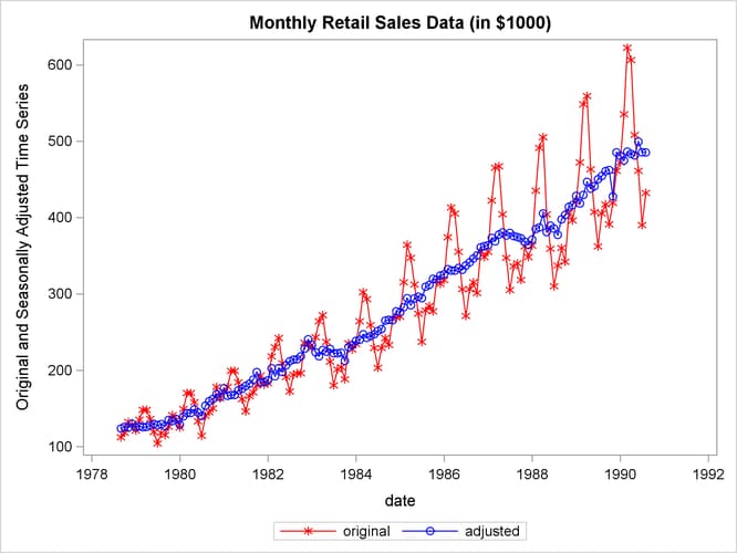
You can compare the original series, table B1, and the final seasonally adjusted series, table D11, by plotting them together. These tables are requested and named in the OUTPUT statement.
title 'Monthly Retail Sales Data (in $1000)';

proc x11 data=sales noprint;
   monthly date=date;
   var sales;
   output out=out b1=sales d11=adjusted;
run;

proc sgplot data=out;
   series x=date y=sales    / markers
                            markerattrs=(color=red symbol='asterisk')
                            lineattrs=(color=red)
                            legendlabel="original" ;
   series x=date y=adjusted / markers
                            markerattrs=(color=blue symbol='circle')
                            lineattrs=(color=blue)
                            legendlabel="adjusted" ;
   yaxis label='Original and Seasonally Adjusted Time Series';
run;
Figure 43.3: Plot of Original and Seasonally Adjusted Data