The HPSEVERITY Procedure

Estimating Regression Effects

Subsections:

Offset Variable
Parameter Initialization for Regression Models
Reporting Estimates of Regression Parameters
CDF and PDF Estimates with Regression Effects

The HPSEVERITY procedure enables you to estimate the influence of regression (exogenous) effects while fitting a distribution if the distribution has a scale parameter or a log-transformed scale parameter.

Let $x_ j$ , $j = 1, \dotsc , k$ , denote the k regression effects. Let $\beta _ j$ denote the regression parameter that corresponds to the effect $x_ j$ . If you do not specify regression effects, then the model for the response variable Y is of the form

$Y \sim \mathcal{F}(\Theta )$

where $\mathcal{F}$ is the distribution of Y with parameters $\Theta$ . This model is usually referred to as the error model. The regression effects are modeled by extending the error model to the following form:

$Y \sim \exp (\sum _{j=1}^{k} \beta _ j x_ j) \cdot \mathcal{F}(\Theta )$

Under this model, the distribution of Y is valid and belongs to the same parametric family as $\mathcal{F}$ if and only if $\mathcal{F}$ has a scale parameter. Let $\theta$ denote the scale parameter and $\Omega$ denote the set of nonscale distribution parameters of $\mathcal{F}$ . Then the model can be rewritten as

$Y \sim \mathcal{F}(\theta , \Omega )$

such that $\theta$ is modeled by the regression effects as

$\theta = \theta _0 \cdot \exp (\sum _{j=1}^{k} \beta _ j x_ j)$

where $\theta _0$ is the base value of the scale parameter. Thus, the scale regression model consists of the following parameters: $\theta _0$ , $\Omega$ , and $\beta _ j (j=1, \dotsc , k)$ .

Given this form of the model, distributions without a scale parameter cannot be considered when regression effects are to be modeled. If a distribution does not have a direct scale parameter, then PROC HPSEVERITY accepts it only if it has a log-transformed scale parameter—that is, if it has a parameter $p = \log (\theta )$ .

Offset Variable

You can specify that an offset variable be included in the scale regression model by specifying it in the OFFSET= option of the SCALEMODEL statement. The offset variable is a regressor whose regression coefficient is known to be 1. If $x_ o$ denotes the offset variable, then the scale regression model becomes

$\theta = \theta _0 \cdot \exp (x_ o + \sum _{j=1}^{k} \beta _ j x_ j)$

The regression coefficient of the offset variable is fixed at 1 and not estimated, so it is not reported in the ParameterEstimates ODS table. However, if you specify the OUTEST= data set, then the regression coefficient is added as a variable to that data set. The value of the offset variable in OUTEST= data set is equal to 1 for the estimates row (_TYPE_='EST') and is equal to a special missing value (.F) for the standard error (_TYPE_='STDERR') and covariance (_TYPE_='COV') rows.

An offset variable is useful to model the scale parameter per unit of some measure of exposure. For example, in the automobile insurance context, measure of exposure can be the number of car-years insured or the total number of miles driven by a fleet of cars at a rental car company. For worker’s compensation insurance, if you want to model the expected loss per enterprise, then you can use the number of employees or total employee salary as the measure of exposure. For epidemiological data, measure of exposure can be the number of people who are exposed to a certain pathogen when you are modeling the loss associated with an epidemic. In general, if e denotes the value of the exposure measure and if you specify $x_ o = \log (e)$ as the offset variable, then you are modeling the influence of other regression effects ( $x_ j$ ) on the size of the scale of the distribution per unit of exposure.

Another use for an offset variable is when you have a priori knowledge of the influence of some exogenous variables that cannot be included in the SCALEMODEL statement. You can model the combined influence of such variables as an offset variable in order to correct for the omitted variable bias.

Parameter Initialization for Regression Models

The regression parameters are initialized either by using the values that you specify or by the default method.

If you provide initial values for the regression parameters, then you must provide valid, nonmissing initial values for $\theta _0$ and $\beta _ j$ parameters for all j.

You can specify the initial value for $\theta _0$ by using either the INEST= data set, the INSTORE= item store, or the INIT= option in the DIST statement. If the distribution has a direct scale parameter (no transformation), then the initial value for the first parameter of the distribution is used as an initial value for $\theta _0$ . If the distribution has a log-transformed scale parameter, then the initial value for the first parameter of the distribution is used as an initial value for $\log (\theta _0)$ .

You can use only the INEST= data set or the INSTORE= item store, but not both, to specify the initial values for $\beta _ j$ . The requirements for each option are as follows:
- If you use the INEST= data set, then it must contain nonmissing initial values for all the regressors that you specify in the SCALEMODEL statement. The only missing value that is allowed is the special missing value .R, which indicates that the regressor is linearly dependent on other regressors. If you specify .R for a regressor for one distribution in a BY group, you must specify it the same way for all the distributions in that BY group.
  
  Note that you cannot specify INEST= data set if the regression model contains effects that have CLASS variables or interaction effects.
- The parameter estimates in the INSTORE= item store are used to initialize the parameters of a model if the item store contains a model specification that matches the model specification in the current PROC HPSEVERITY step according to the following rules:
  - The distribution name and the number and names of the distribution parameters must match.
  - The model in the item store must include a scale regression model whose regression parameters match as follows:
    
    If the regression model in the item store does not contain any redundant parameters, then at least one regression parameter must match. Initial values of the parameters that match are set equal to the estimates that are read from the item store, and initial values of the other regression parameters are set equal to the default value of 0.001.
    
    If the regression model in the item store contains any redundant parameters, then all the regression parameters must match, and the initial values of all parameters are set equal to the estimates that are read from the item store.
    
    Note that a regression parameter is defined by the variables that form the underlying regression effect and by the levels of the CLASS variables if the effect contains any CLASS variables.
If you do not specify valid initial values for $\theta _0$ or $\beta _ j$ parameters for all j, then PROC HPSEVERITY initializes those parameters by using the following method:

Let a random variable Y be distributed as $\mathcal{F}(\theta , \Omega )$ , where $\theta$ is the scale parameter. By the definition of the scale parameter, a random variable $W = Y/\theta$ is distributed as $\mathcal{G}(\Omega )$ such that $\mathcal{G}(\Omega ) = \mathcal{F}(1, \Omega )$ . Given a random error term e that is generated from a distribution $\mathcal{G}(\Omega )$ , a value y from the distribution of Y can be generated as

$y = \theta \cdot e$

Taking the logarithm of both sides and using the relationship of $\theta$ with the regression effects yields:

$\log (y) = \log (\theta _0) + \sum _{j=1}^{k} \beta _ j x_ j + \log (e)$

PROC HPSEVERITY makes use of the preceding relationship to initialize parameters of a regression model with distribution dist as follows:
1. The following linear regression problem is solved to obtain initial estimates of $\beta _0$ and $\beta _ j$ :
  
  $\log (y) = \beta _0 + \sum _{j=1}^{k} \beta _ j x_ j$
  
  The estimates of $\beta _ j (j=1, \dotsc , k)$ in the solution of this regression problem are used to initialize the respective regression parameters of the model. The estimate of $\beta _0$ is later used to initialize the value of $\theta _0$ .
  
  The results of this regression are also used to detect whether any regression parameters are linearly dependent on the other regression parameters. If any such parameters are found, then a warning is written to the SAS log and the corresponding parameter is eliminated from further analysis. The estimates for linearly dependent regression parameters are denoted by a special missing value of .R in the OUTEST= data set and in any displayed output.
2. Let $s_0$ denote the initial value of the scale parameter.
  
  If the distribution model of dist does not contain the dist_PARMINIT subroutine, then $s_0$ and all the nonscale distribution parameters are initialized to the default value of 0.001.
  
  However, it is strongly recommended that each distribution’s model contain the dist_PARMINIT subroutine. For more information, see the section Defining a Severity Distribution Model with the FCMP Procedure. If that subroutine is defined, then $s_0$ is initialized as follows:
  
  Each input value $y_ i$ of the response variable is transformed to its scale-normalized version $w_ i$ as
  
  $w_ i = \frac{y_ i}{\exp (\beta _0 + \sum _{j=1}^{k} \beta _ j x_{ij})}$
  
  where $x_{ij}$ denotes the value of jth regression effect in the ith input observation. These $w_ i$ values are used to compute the input arguments for the dist_PARMINIT subroutine. The values that are computed by the subroutine for nonscale parameters are used as their respective initial values. If the distribution has an untransformed scale parameter, then $s_0$ is set to the value of the scale parameter that is computed by the subroutine. If the distribution has a log-transformed scale parameter P, then $s_0$ is computed as $s_0 = \exp (l_0)$ , where $l_0$ is the value of P computed by the subroutine.
3. The value of $\theta _0$ is initialized as
  
  $\theta _0 = s_0 \cdot \exp (\beta _0)$

Reporting Estimates of Regression Parameters

When you request estimates to be written to the output (either ODS displayed output or in the OUTEST= data set), the estimate of the base value of the first distribution parameter is reported. If the first parameter is the log-transformed scale parameter, then the estimate of $\log (\theta _0)$ is reported; otherwise, the estimate of $\theta _0$ is reported. The transform of the first parameter of a distribution dist is controlled by the dist_SCALETRANSFORM function that is defined for it.

CDF and PDF Estimates with Regression Effects

When regression effects are estimated, the estimate of the scale parameter depends on the values of the regressors and the estimates of the regression parameters. This dependency results in a potentially different distribution for each observation. To make estimates of the cumulative distribution function (CDF) and probability density function (PDF) comparable across distributions and comparable to the empirical distribution function (EDF), PROC HPSEVERITY computes and reports the CDF and PDF estimates from a representative distribution. The representative distribution is a mixture of a certain number of distributions, where each distribution differs only in the value of the scale parameter. You can specify the number of distributions in the mixture and how their scale values are chosen by using the DFMIXTURE= option in the SCALEMODEL statement.

Let N denote the number of observations that are used for estimation, K denote the number of components in the mixture distribution, $s_ k$ denote the scale parameter of the kth mixture component, and $d_ k$ denote the weight associated with kth mixture component.

Let $f(y; s_ k,\hat{\Omega })$ and $F(y; s_ k,\hat{\Omega })$ denote the PDF and CDF, respectively, of the kth component distribution, where $\hat{\Omega }$ denotes the set of estimates of all parameters of the distribution other than the scale parameter. Then, the PDF and CDF estimates, $f^{*}(y)$ and $F^{*}(y)$ , respectively, of the mixture distribution at y are computed as

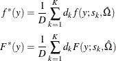
$\begin{align*} f^{*}(y) & = \frac{1}{D} \sum _{k=1}^{K} d_ k f(y; s_ k, \hat{\Omega }) \\ F^{*}(y) & = \frac{1}{D} \sum _{k=1}^{K} d_ k F(y; s_ k, \hat{\Omega }) \end{align*}$

where D is the normalization factor ( $D = \sum _{k=1}^{K} d_ k$ ).

PROC HPSEVERITY uses the $F^{*}(y)$ values to compute the EDF-based statistics of fit and to create the OUTCDF= data set and the CDF plots. The PDF estimates that it plots in the PDF plots are the $f^{*}(y)$ values.

The scale values $s_ k$ for the K mixture components are derived from the set $\{ \hat{\lambda }_ i\}$ ( $i=1, \ldots , N$ ) of N linear predictor values, where $\hat{\lambda }_ i$ denotes the estimate of the linear predictor due to observation i. It is computed as

$\hat{\lambda }_ i = \log (\hat{\theta }_0) + \sum _{j=1}^{k} \hat{\beta }_ j x_{ij}$

where $\hat{\theta }_0$ is an estimate of the base value of the scale parameter, $\hat{\beta }_ j$ are the estimates of regression coefficients, and $x_{ij}$ is the value of jth regression effect in observation i.

Let $w_ i$ denote the weight of observation i. If you specify the WEIGHT statement, then the weight is equal to the value of the specified weight variable for the corresponding observation in the DATA= data set; otherwise, the weight is set to 1.

You can specify one of the following method-names in the DFMIXTURE= option in the SCALEMODEL statement to specify the method of choosing K and the corresponding $s_ k$ and $d_ k$ values:

FULL

In this method, there are as many mixture components as the number of observations that are used for estimation. In other words, K = N, $s_ k = \hat{\theta }_ k$ , and $d_ k = w_ k$ ( $k=1, \ldots , N$ ). This is the slowest method, because it requires $O(N)$ computations to compute the mixture CDF $F^{*}(y_ i)$ or the mixture PDF $f^{*}(y_ i)$ of one observation. For N observations, the computational complexity in terms of number of CDF or PDF evaluations is $O(N^2)$ . Even for moderately large values of N, the time that is taken to compute the mixture CDF and PDF can significantly exceed the time that is taken to estimate the model parameters. So it is recommended that you use the FULL method only for small data sets.

MEAN

In this method, the mixture contains only one distribution, whose scale value is determined by the mean of the linear predictor values that are implied by all the observations. In other words, $s_1$ is computed as

$s_1 = \exp \left(\frac{1}{N} \sum _{i=1}^{N} \hat{\lambda }_ i \right)$

The component’s weight $d_1$ is set to 1.

This method is the fastest because it requires only one CDF or PDF evaluation per observation. The computational complexity is $O(N)$ for N observations.

If you do not specify the DFMIXTURE= option in the SCALEMODEL statement, then this is the default method.

QUANTILE

In this method, a certain number of quantiles are chosen from the set of all linear predictor values. If you specify a value of $\Argument{q}$ for the K= option when specifying this method, then $K=\Argument{q}-1$ and $s_ k$ ( $k=1, \ldots , K$ ) is computed as $s_ k = \exp (\hat{\lambda }_ k)$ , where $\hat{\lambda }_ k$ is the kth $\Argument{q}$ -quantile from the set $\{ \hat{\lambda }_ i\}$ ( $i=1, \ldots , N$ ). The weight of each of the components ( $d_ k$ ) is assumed to be 1 for this method.

The default value of $\Argument{q}$ is 2, which implies a one-point mixture that has a distribution whose scale value is equal to the median scale value.

For this method, PROC HPSEVERITY needs to sort the N linear predictor values in the set $\{ \hat{\lambda }_ i\}$ ; the sorting requires $O(N \log (N))$ computations. Then, computing the mixture estimate of one observation requires $(\Argument{q}-1)$ CDF or PDF evaluations. Hence, the computational complexity of this method is $O(qN)+O(N \log (N))$ for computing a mixture CDF or PDF of N observations. For $\Argument{q} << N$ , the QUANTILE method is significantly faster than the FULL method.

RANDOM

In this method, a uniform random sample of observations is chosen, and the mixture contains the distributions that are implied by those observations. If you specify a value of $\Argument{r}$ for the K= option when specifying this method, then the size of the sample is $\Argument{r}$ . Hence, $K=\Argument{r}$ . If $l_ j$ denotes the index of jth observation in the sample ( $j=1, \ldots , \Argument{r}$ ), such that $1 \le l_ j \le N$ , then the scale of kth component distribution in the mixture is $s_ k = \exp (\hat{\lambda }_{l_ k})$ . The weight of each of the components ( $d_ k$ ) is assumed to be 1 for this method.

You can also specify the seed to be used for generating the random sample by using the SEED= option for this method. The same sample of observations is used for all models.

Computing a mixture estimate of one observation requires $\Argument{r}$ CDF or PDF evaluations. Hence, the computational complexity of this method is $O(\Argument{r}N)$ for computing a mixture CDF or PDF of N observations. For $\Argument{r} << N$ , the RANDOM method is significantly faster than the FULL method.