The HPSEVERITY Procedure
- Overview
-
Getting Started

-
Syntax
-
DetailsPredefined DistributionsCensoring and TruncationParameter Estimation MethodParameter InitializationEstimating Regression EffectsLevelization of Classification VariablesSpecification and Parameterization of Model EffectsEmpirical Distribution Function Estimation MethodsStatistics of FitDistributed and Multithreaded ComputationDefining a Severity Distribution Model with the FCMP ProcedurePredefined Utility FunctionsScoring FunctionsCustom Objective FunctionsInput Data SetsOutput Data SetsDisplayed OutputODS Graphics
-
ExamplesDefining a Model for Gaussian DistributionDefining a Model for the Gaussian Distribution with a Scale ParameterDefining a Model for Mixed-Tail DistributionsFitting a Scaled Tweedie Model with RegressorsFitting Distributions to Interval-Censored DataBenefits of Distributed and Multithreaded ComputingEstimating Parameters Using Cramér-von Mises EstimatorDefining a Finite Mixture Model That Has a Scale ParameterPredicting Mean and Value-at-Risk by Using Scoring FunctionsScale Regression with Rich Regression Effects
- References
Predefined Distributions
PROC HPSEVERITY assumes the following model for the response variable Y
![\[ Y \sim \mathcal{F}(\Theta ) \]](images/etsug_hpseverity0038.png)
where  is a continuous probability distribution with parameters
  . The model hypothesizes that the observed response is generated from a stochastic process that is governed by the distribution
. This model is usually referred to as the error model. Given a representative input sample of response variable values, PROC
HPSEVERITY estimates the model parameters for any distribution and computes the statistics of fit for each model. This enables you to find the distribution that is most likely to generate
the observed sample.
. The model hypothesizes that the observed response is generated from a stochastic process that is governed by the distribution
. This model is usually referred to as the error model. Given a representative input sample of response variable values, PROC
HPSEVERITY estimates the model parameters for any distribution and computes the statistics of fit for each model. This enables you to find the distribution that is most likely to generate
the observed sample.
A set of predefined distributions is provided with the HPSEVERITY procedure. A summary of the distributions is provided in Table 23.2. For each distribution, the table lists the name of the distribution that should be used in the DIST statement, the parameters of the distribution along with their bounds, and the mathematical expressions for the probability density function (PDF) and cumulative distribution function (CDF) of the distribution.
All the predefined distributions, except LOGN and TWEEDIE, are parameterized such that their first parameter is the scale
parameter. For LOGN, the first parameter  is a log-transformed scale parameter. TWEEDIE does not have a scale parameter. The presence of scale parameter or a log-transformed
scale parameter enables you to use all of the predefined distributions, except TWEEDIE, as a candidate for estimating regression
effects.
is a log-transformed scale parameter. TWEEDIE does not have a scale parameter. The presence of scale parameter or a log-transformed
scale parameter enables you to use all of the predefined distributions, except TWEEDIE, as a candidate for estimating regression
effects.
A distribution model is associated with each predefined distribution. You can also define your own distribution model, which is a set of functions and subroutines that you define by using the FCMP procedure. For more information, see the section Defining a Severity Distribution Model with the FCMP Procedure.
Table 23.2: Predefined HPSEVERITY Distributions
|
Name |
Distribution |
Parameters |
PDF (f) and CDF (F) |
|
|---|---|---|---|---|
|
BURR |
Burr |
|
|
|
|
|
|
|
||
|
EXP |
Exponential |
|
|
|
|
|
|
|||
|
GAMMA |
Gamma |
|
|
|
|
|
|
|||
|
GPD |
Generalized |
|
|
|
|
Pareto |
|
|
||
|
IGAUSS |
Inverse Gaussian |
|
|
|
|
(Wald) |
|
|
||
|
|
||||
|
LOGN |
Lognormal |
|
|
|
|
|
|
|
||
|
PARETO |
Pareto |
|
|
|
|
|
|
|||
|
TWEEDIE |
Tweedie |
|
|
|
|
|
|
|
||
|
STWEEDIE |
Scaled Tweedie |
|
|
|
|
|
|
|
||
|
WEIBULL |
Weibull |
|
|
|
|
|
|
|||
|
Notes: |
||||
|
1. |
||||
|
2. |
||||
|
3. Parameters are listed in the order in which they are defined in the distribution model. |
||||
|
4. |
||||
|
5. |
||||
|
6. For more information, see the section Tweedie Distributions. |
||||


![$a(x,\phi ) \exp \left[ \frac{1}{\phi } \left( \frac{x \mu ^{1-p}}{1-p} - \kappa (\mu ,p) \right) \right]$](images/etsug_hpseverity0064.png)


Tweedie Distributions
Tweedie distributions are a special case of the exponential dispersion family (Jørgensen 1987) with a property that the variance of the distribution is equal to  , where is the mean of the distribution,
  is a dispersion parameter, and p is an index parameter as discovered by Tweedie (1984). The distribution is defined for all values of p except for values of p in the open interval
  . Many important known distributions are a special case of Tweedie distributions including normal (p=0), Poisson (p=1), gamma (p=2), and the inverse Gaussian (p=3). Apart from these special cases, the probability density function (PDF) of the Tweedie distribution does not have an analytic
expression. For
. Many important known distributions are a special case of Tweedie distributions including normal (p=0), Poisson (p=1), gamma (p=2), and the inverse Gaussian (p=3). Apart from these special cases, the probability density function (PDF) of the Tweedie distribution does not have an analytic
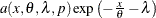
expression. For  , it has the form (Dunn and Smyth 2005),
![\[ f(x; \mu , \phi , p) = a(x,\phi ) \exp \left[ \frac{1}{\phi } \left( \frac{x \mu ^{1-p}}{1-p} - \kappa (\mu ,p) \right) \right] \]](images/etsug_hpseverity0080.png)
where  for
for  and
and  for p = 2. The function
  does not have an analytical expression. It is typically evaluated using series expansion methods described in Dunn and Smyth
(2005).
does not have an analytical expression. It is typically evaluated using series expansion methods described in Dunn and Smyth
(2005).
For  , the Tweedie distribution is a compound Poisson-gamma mixture distribution, which is the distribution of S defined as
![\[ S = \sum _{i=1}^{N} X_ i \]](images/etsug_hpseverity0085.png)
where  and
and 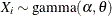 are independent and identically distributed gamma random variables with shape parameter
  and scale parameter
  . At X = 0, the density is a probability mass that is governed by the Poisson distribution, and for values of
  , it is a mixture of gamma variates with Poisson mixing probability. The parameters
  , , and are related to the natural parameters , , and p of the Tweedie distribution as
The mean of a Tweedie distribution is positive for .
Two predefined versions of the Tweedie distribution are provided with the HPSEVERITY procedure. The first version, named TWEEDIE
and defined for , has the natural parameterization with parameters , , and p. The second version, named STWEEDIE and defined for , is the version with a scale parameter. It corresponds to the compound Poisson-gamma distribution with gamma scale parameter
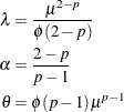
, Poisson mean parameter , and the index parameter p. The index parameter decides the shape parameter of the gamma distribution as
![\[ \alpha = \frac{2-p}{p-1} \]](images/etsug_hpseverity0091.png)
The parameters and of the STWEEDIE distribution are related to the parameters and of the TWEEDIE distribution as
You can fit either version when there are no regression variables. Each version has its own merits. If you fit the TWEEDIE
version, you have the direct estimate of the overall mean of the distribution. If you are interested in the most practical
range of the index parameter , then you can fit the STWEEDIE version, which provides you direct estimates of the Poisson and gamma components that comprise
the distribution (an estimate of the gamma shape parameter is easily obtained from the estimate of p).
If you want to estimate the effect of exogenous (regression) variables on the distribution, then you must use the STWEEDIE
version, because PROC HPSEVERITY requires a distribution to have a scale parameter in order to estimate regression effects.
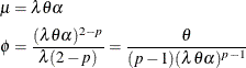
For more information, see the section Estimating Regression Effects. The gamma scale parameter is the scale parameter of the STWEEDIE distribution. If you are interested in determining the effect of regression variables
on the mean of the distribution, you can do so by first fitting the STWEEDIE distribution to determine the effect of the regression
variables on the scale parameter . Then, you can easily estimate how the mean of the distribution is affected by the regression variables using the relationship  , where
  . The estimates of the regression parameters remain the same, whereas the estimate of the intercept parameter is adjusted
by the estimates of the and p parameters.
. The estimates of the regression parameters remain the same, whereas the estimate of the intercept parameter is adjusted
by the estimates of the and p parameters.
Parameter Initialization for Predefined Distributions
The parameters are initialized by using the method of moments for all the distributions, except for the gamma and the Weibull distributions. For the gamma distribution, approximate maximum likelihood estimates are used. For the Weibull distribution, the method of percentile matching is used.
Given n observations of the severity value  (
( ), the estimate of kth raw moment is denoted by
  and computed as
![\[ m_ k = \frac{1}{n} \sum _{i=1}^{n} y_ i^ k \]](images/etsug_hpseverity0098.png)
The 100pth percentile is denoted by  (
( ). By definition, satisfies
![\[ F(\pi _ p-) \le p \le F(\pi _ p) \]](images/etsug_hpseverity0101.png)
where 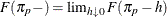 . PROC HPSEVERITY uses the following practical method of computing . Let
  denote the empirical distribution function (EDF) estimate at a severity value y. Let
  and
and  denote two consecutive values in the ascending sequence of y values such that
  and
and  . Then, the estimate
  is computed as
![\[ \hat{\pi }_ p = y_ p^- + \frac{p - \hat{F}_ n(y_ p^-)}{\hat{F}_ n(y_ p^+) - \hat{F}_ n(y_ p^-)} (y_ p^+ - y_ p^-) \]](images/etsug_hpseverity0109.png)
Let  denote the smallest double-precision floating-point number such that
  . This machine precision constant can be obtained by using the CONSTANT function in Base SAS software.
The details of how parameters are initialized for each predefined distribution are as follows:
- BURR
-
The parameters are initialized by using the method of moments. The kth raw moment of the Burr distribution is:
![\[ E[X^ k] = \frac{\theta ^ k \Gamma (1 + k/\gamma ) \Gamma (\alpha - k/\gamma )}{\Gamma (\alpha )}, \quad -\gamma < k < \alpha \gamma \]](images/etsug_hpseverity0112.png)
Three moment equations
![$E[X^ k] = m_ k$](images/etsug_hpseverity0113.png) (
( ) need to be solved for initializing the three parameters of the distribution. In order to get an approximate closed form
solution, the second shape parameter
) need to be solved for initializing the three parameters of the distribution. In order to get an approximate closed form
solution, the second shape parameter  is initialized to a value of 2. If
  , then simplifying and solving the moment equations yields the following feasible set of initial values:
![\[ \hat{\theta } = \sqrt {\frac{m_2 m_3}{2 m_3 - 3 m_1 m_2}}, \quad \hat{\alpha } = 1 + \frac{m_3}{2 m_3 - 3 m_1 m_2}, \quad \hat{\gamma } = 2 \]](images/etsug_hpseverity0117.png)
If
 , then the parameters are initialized as follows:
![\[ \hat{\theta } = \sqrt {m_2}, \quad \hat{\alpha } = 2, \quad \hat{\gamma } = 2 \]](images/etsug_hpseverity0119.png)
- EXP
-
The parameters are initialized by using the method of moments. The kth raw moment of the exponential distribution is:
![\[ E[X^ k] = \theta ^ k \Gamma (k+1), \quad k > -1 \]](images/etsug_hpseverity0120.png)
Solving
![$E[X] = m_1$](images/etsug_hpseverity0121.png) yields the initial value of
yields the initial value of  .
.
- GAMMA
-
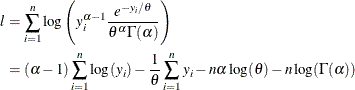
The parameter
is initialized by using its approximate maximum likelihood (ML) estimate. For a set of n independent and identically distributed observations () drawn from a gamma distribution, the log likelihood l is defined as follows:
Using a shorter notation of
 to denote
  and solving the equation
  yields the following ML estimate of :
![\[ \hat{\theta } = \frac{\sum y_ i}{n \alpha } = \frac{m_1}{\alpha } \]](images/etsug_hpseverity0127.png)
Substituting this estimate in the expression of l and simplifying gives
![\[ l = (\alpha - 1) \sum \log (y_ i) - n \alpha - n \alpha \log (m_1) + n \alpha \log (\alpha ) - n \log (\Gamma (\alpha )) \]](images/etsug_hpseverity0128.png)
Let d be defined as follows:
![\[ d = \log (m_1) - \frac{1}{n} \sum \log (y_ i) \]](images/etsug_hpseverity0129.png)
Solving the equation
 yields the following expression in terms of the digamma function,
  :
:
![\[ \log (\alpha ) - \psi (\alpha ) = d \]](images/etsug_hpseverity0132.png)
The digamma function can be approximated as follows:
![\[ \hat{\psi }(\alpha ) \approx \log (\alpha ) - \frac{1}{\alpha } \left(0.5 + \frac{1}{12 \alpha + 2}\right) \]](images/etsug_hpseverity0133.png)
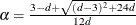
This approximation is within 1.4% of the true value for all the values of
 except when is arbitrarily close to the positive root of the digamma function (which is approximately 1.461632). Even for the values
of that are close to the positive root, the absolute error between true and approximate values is still acceptable (
except when is arbitrarily close to the positive root of the digamma function (which is approximately 1.461632). Even for the values
of that are close to the positive root, the absolute error between true and approximate values is still acceptable ( for
for  ). Solving the equation that arises from this approximation yields the following estimate of :
![\[ \hat{\alpha } = \frac{3 - d + \sqrt {(d-3)^2 + 24 d}}{12 d} \]](images/etsug_hpseverity0136.png)
If this approximate ML estimate is infeasible, then the method of moments is used. The kth raw moment of the gamma distribution is:
![\[ E[X^ k] = \theta ^ k \frac{\Gamma (\alpha + k)}{\Gamma (\alpha )}, \quad k > -\alpha \]](images/etsug_hpseverity0137.png)
Solving
and ![$E[X^2] = m_2$](images/etsug_hpseverity0138.png) yields the following initial value for :
yields the following initial value for :
![\[ \hat{\alpha } = \frac{m_1^2}{m_2 - m_1^2} \]](images/etsug_hpseverity0139.png)
If
 (almost zero sample variance), then is initialized as follows:
![\[ \hat{\alpha } = 1 \]](images/etsug_hpseverity0141.png)
After computing the estimate of
, the estimate of is computed as follows:
![\[ \hat{\theta } = \frac{m_1}{\hat{\alpha }} \]](images/etsug_hpseverity0142.png)
Both the maximum likelihood method and the method of moments arrive at the same relationship between
 and
and  .
.
- GPD
-
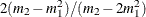
The parameters are initialized by using the method of moments. Notice that for
 , the CDF of the generalized Pareto distribution (GPD) is:
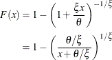
This is equivalent to a Pareto distribution with scale parameter
 and shape parameter
  . Using this relationship, the parameter initialization method used for the PARETO distribution is used to get the following
initial values for the parameters of the GPD distribution:
. Using this relationship, the parameter initialization method used for the PARETO distribution is used to get the following
initial values for the parameters of the GPD distribution:
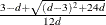
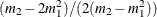
![\[ \hat{\theta } = \frac{m_1 m_2}{2 (m_2 - m_1^2)}, \quad \hat{\xi } = \frac{m_2 - 2 m_1^2}{2 (m_2 - m_1^2)} \]](images/etsug_hpseverity0148.png)
If
(almost zero sample variance) or  , then the parameters are initialized as follows:
![\[ \hat{\theta } = \frac{m_1}{2}, \quad \hat{\xi } = \frac{1}{2} \]](images/etsug_hpseverity0150.png)
- IGAUSS
-
The parameters are initialized by using the method of moments. The standard parameterization of the inverse Gaussian distribution (also known as the Wald distribution), in terms of the location parameter
and shape parameter , is as follows (Klugman, Panjer, and Willmot 1998, p. 583):
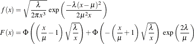
For this parameterization, it is known that the mean is
![$E[X] = \mu $](images/etsug_hpseverity0152.png) and the variance is
and the variance is ![$Var[X] = \mu ^3/\lambda $](images/etsug_hpseverity0153.png) , which yields the second raw moment as
, which yields the second raw moment as ![$E[X^2] = \mu ^2 (1 + \mu /\lambda )$](images/etsug_hpseverity0154.png) (computed by using
(computed by using ![$E[X^2] = Var[X] + (E[X])^2$](images/etsug_hpseverity0155.png) ).
).
The predefined IGAUSS distribution in PROC HPSEVERITY uses the following alternate parameterization to allow the distribution to have a scale parameter,
:
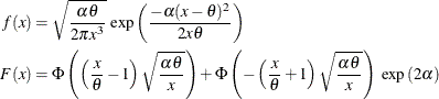
The parameters
(scale) and (shape) of this alternate form are related to the parameters and of the preceding form such that  and
and  . Using this relationship, the first and second raw moments of the IGAUSS distribution are:
![\begin{align*} E[X] & = \theta \\ E[X^2] & = \theta ^2 \left(1 + \frac{1}{\alpha }\right) \end{align*}](images/etsug_hpseverity0159.png)
Solving
and yields the following initial values:
![\[ \hat{\theta } = m_1, \quad \hat{\alpha } = \frac{m_1^2}{m_2 - m_1^2} \]](images/etsug_hpseverity0160.png)
If
(almost zero sample variance), then the parameters are initialized as follows:
![\[ \hat{\theta } = m_1, \quad \hat{\alpha } = 1 \]](images/etsug_hpseverity0161.png)
- LOGN
-
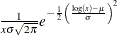
The parameters are initialized by using the method of moments. The kth raw moment of the lognormal distribution is:
![\[ E[X^ k] = \exp \left(k \mu + \frac{k^2 \sigma ^2}{2}\right) \]](images/etsug_hpseverity0162.png)
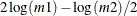
Solving
and yields the following initial values:
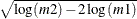
![\[ \hat{\mu } = 2 \log (m1) - \frac{\log (m2)}{2}, \quad \hat{\sigma } = \sqrt {\log (m2) - 2 \log (m1)} \]](images/etsug_hpseverity0163.png)
- PARETO
-
The parameters are initialized by using the method of moments. The kth raw moment of the Pareto distribution is:
![\[ E[X^ k] = \frac{\theta ^ k \Gamma (k + 1) \Gamma (\alpha - k)}{\Gamma (\alpha )}, -1 < k < \alpha \]](images/etsug_hpseverity0164.png)
Solving
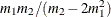
and yields the following initial values:
![\[ \hat{\theta } = \frac{m_1 m_2}{m_2 - 2 m_1^2}, \quad \hat{\alpha } = \frac{2(m_2 - m_1^2)}{m_2 - 2 m_1^2} \]](images/etsug_hpseverity0165.png)
If
(almost zero sample variance) or , then the parameters are initialized as follows:
![\[ \hat{\theta } = m_1, \quad \hat{\alpha } = 2 \]](images/etsug_hpseverity0166.png)
- TWEEDIE
-
The parameter p is initialized by assuming that the sample is generated from a gamma distribution with shape parameter
and by computing  . The initial value is obtained from using the method previously described for the GAMMA distribution. The parameter is the mean of the distribution. Hence, it is initialized to the sample mean as
![\[ \hat{\mu } = m_1 \]](images/etsug_hpseverity0168.png)
Variance of a Tweedie distribution is equal to
. Thus, the sample variance is used to initialize the value of as
![\[ \hat{\phi } = \frac{m_2 - m_1^2}{\hat{\mu }^{\hat{p}}} \]](images/etsug_hpseverity0169.png)
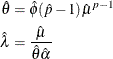
- STWEEDIE
-
STWEEDIE is a compound Poisson-gamma mixture distribution with mean
 , where is the shape parameter of the gamma random variables in the mixture and the parameter p is determined solely by . First, the parameter p is initialized by assuming that the sample is generated from a gamma distribution with shape parameter and by computing . The initial value is obtained from using the method previously described for the GAMMA distribution. As done for initializing the parameters
of the TWEEDIE distribution, the sample mean and variance are used to compute the values
, where is the shape parameter of the gamma random variables in the mixture and the parameter p is determined solely by . First, the parameter p is initialized by assuming that the sample is generated from a gamma distribution with shape parameter and by computing . The initial value is obtained from using the method previously described for the GAMMA distribution. As done for initializing the parameters
of the TWEEDIE distribution, the sample mean and variance are used to compute the values  and
and  as
as

Based on the relationship between the parameters of TWEEDIE and STWEEDIE distributions described in the section Tweedie Distributions, values of
and are initialized as
- WEIBULL
-
The parameters are initialized by using the percentile matching method. Let
 and
and  denote the estimates of the 25th and 75th percentiles, respectively. Using the formula for the CDF of Weibull distribution,
they can be written as
denote the estimates of the 25th and 75th percentiles, respectively. Using the formula for the CDF of Weibull distribution,
they can be written as
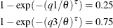
Simplifying and solving these two equations yields the following initial values:
![\[ \hat{\theta } = \exp \left(\frac{r \log (q1) - \log (q3)}{r - 1}\right), \quad \hat{\tau } = \frac{\log (\log (4))}{\log (q3) - \log (\hat{\theta })} \]](images/etsug_hpseverity0178.png)
where
 . These initial values agree with those suggested in Klugman, Panjer, and Willmot (1998).
A summary of the initial values of all the parameters for all the predefined distributions is given in Table 23.3. The table also provides the names of the parameters to use in the INIT= option in the DIST statement if you want to provide a different initial value.
Table 23.3: Parameter Initialization for Predefined Distributions
|
Distribution |
Parameter |
Name for INIT option |
Default Initial Value |
|---|---|---|---|
|
BURR |
|
theta |
|
|
|
alpha |
|
|
|
|
gamma |
2 |
|
|
EXP |
|
theta |
|
|
GAMMA |
|
theta |
|
|
|
alpha |
|
|
|
GPD |
|
theta |
|
|
|
xi |
|
|
|
IGAUSS |
|
theta |
|
|
|
alpha |
|
|
|
LOGN |
|
mu |
|
|
|
sigma |
|
|
|
PARETO |
|
theta |
|
|
|
alpha |
|
|
|
TWEEDIE |
|
mu |
|
|
|
phi |
|
|
|
p |
p |
|
|
|
where |
|||
|
STWEEDIE |
|
theta |
|
|
|
lambda |
|
|
|
p |
p |
|
|
|
where |
|||
|
WEIBULL |
|
theta |
|
|
|
tau |
|
|
|
Notes: |
|||
|
|
|||
|
|
|||
|
|
|||
|
|
|||