The ENTROPY Procedure(Experimental)
- Overview
-
Getting Started

-
Syntax
-
DetailsGeneralized Maximum EntropyGeneralized Cross EntropyMoment Generalized Maximum EntropyMaximum Entropy-Based Seemingly Unrelated RegressionGeneralized Maximum Entropy for Multinomial Discrete Choice ModelsCensored or Truncated Dependent VariablesInformation MeasuresParameter Covariance For GCEParameter Covariance For GCE-MStatistical TestsMissing ValuesInput Data SetsOutput Data SetsODS Table NamesODS Graphics
-
Examples
- References
Pure Inverse Problems
A special case of systems of equations estimation is the pure inverse problem. A pure problem is one that contains an exact relationship between the dependent variable and the independent variables and does not have an error component. A pure inverse problem can be written as
![\[ \mb{y} = X \beta \]](images/etsug_entropy0014.png)
where  is a n-dimensional vector of observations,
  is a
is a  matrix of regressors, and
  is a k-dimensional vector of unknowns. Notice that there is no error term.
A classic example is a dice problem (Jaynes 1963). Given a six-sided die that can take on the values  and the average outcome of the die
  , compute the probabilities
 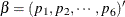 of rolling each number. This infers six values from two pieces of information. The data points are the expected value of
y, and the sum of the probabilities is one. Given
of rolling each number. This infers six values from two pieces of information. The data points are the expected value of
y, and the sum of the probabilities is one. Given  , this problem is solved by using the following SAS code:
data one;
   array x[6] ( 1 2 3 4 5 6 );
   y=4.0;
run;
proc entropy data=one pure;
   priors x1 0 1 x2 0 1 x3 0 1 x4 0 1 x5 0 1 x6 0 1;
   model y = x1-x6/ noint;
   restrict x1 + x2 +x3 +x4 + x5 + x6 =1;
run;
The probabilities are given in Figure 14.16.
Figure 14.16: Jaynes’ Dice Pure Inverse Problem
Note how the probabilities are skewed to the higher values because of the high average roll provided in the input data.
First-Order Markov Process Estimation
A more useful inverse problem is the first-order markov process. Companies have a share of the marketplace where they do business. Generally, customers for a specific market space can move from company to company. The movement of customers can be visualized graphically as a flow diagram, as in Figure 14.17. The arrows represent movements of customers from one company to another.
Figure 14.17: Markov Transition Diagram
You can model the probability that a customer moves from one company to another using a first-order Markov model. Mathematically the model is:
![\[ y_ t = P y_{t-1} \]](images/etsug_entropy0021.png)
where  is a vector of k market shares at time t and P is a
  matrix of unknown transition probabilities. The value
  represents the probability that a customer who is currently using company j at time
  moves to company i at time t. The diagonal elements then represent the probability that a customer stays with the current company. The columns in P sum to one.
Given market share information over time, you can estimate the transition probabilities P. In order to estimate P using traditional methods, you need at least k observations. If you have fewer than k transitions, you can use the ENTROPY procedure to estimate the probabilities.
Suppose you are studying the market share for four companies. If you want to estimate the transition probabilities for these four companies, you need a time series with four observations of the shares. Assume the current transition probability matrix is as follows:
![\[ \left[ \begin{array}{cccc} 0.7 & 0.4 & 0.0 & 0.1 \\ 0.1 & 0.5 & 0.4 & 0.0 \\ 0.0 & 0.1 & 0.6 & 0.0 \\ 0.2 & 0.0 & 0.0 & 0.9 \end{array} \right] \]](images/etsug_entropy0026.png)
The following SAS DATA step statements generate a series of market shares from this probability matrix. A transition is represented
as the current period shares, y, and the previous period shares, x.
data m;
            /* Known Transition matrix */
   array p[4,4] (0.7 .4 .0 .1
                 0.1 .5 .4 .0
                 0.0 .1 .6 .0
                 0.2 .0 .0 .9 ) ;
            /* Initial Market shares */
   array y[4] y1-y4 ( .4 .3 .2 .1 );
   array x[4] x1-x4;
   drop p1-p16 i;
   do i = 1 to 3;
       x[1] = y[1]; x[2] = y[2];
       x[3] = y[3]; x[4] = y[4];
       y[1] = p[1,1] * x1 + p[1,2] * x2 + p[1,3] * x3 + p[1,4] * x4;
       y[2] = p[2,1] * x1 + p[2,2] * x2 + p[2,3] * x3 + p[2,4] * x4;
       y[3] = p[3,1] * x1 + p[3,2] * x2 + p[3,3] * x3 + p[3,4] * x4;
       y[4] = p[4,1] * x1 + p[4,2] * x2 + p[4,3] * x3 + p[4,4] * x4;
       output;
   end;
run;
The following SAS statements estimate the transition matrix by using only the first transition.
proc entropy markov pure data=m(obs=1);
   model y1-y4 = x1-x4;
run;
The MARKOV option implies NOINT for each model, that the sum of the parameters in each column is one, and chooses support points of 0 and 1. This model can be expressed equivalently as
proc entropy pure data=m(obs=1) ;
   priors y1.x1 0 1 y1.x2 0 1 y1.x3 0 1 y1.x4 0 1;
   priors y2.x1 0 1 y2.x2 0 1 y2.x3 0 1 y2.x4 0 1;
   priors y3.x1 0 1 y3.x2 0 1 y3.x3 0 1 y3.x4 0 1;
   priors y4.x1 0 1 y4.x2 0 1 y4.x3 0 1 y4.x4 0 1;

   model y1 = x1-x4 / noint;
   model y2 = x1-x4 / noint;
   model y3 = x1-x4 / noint;
   model y4 = x1-x4 / noint;

   restrict y1.x1 + y2.x1 + y3.x1 + y4.x1 = 1;
   restrict y1.x2 + y2.x2 + y3.x2 + y4.x2 = 1;
   restrict y1.x3 + y2.x3 + y3.x3 + y4.x3 = 1;
   restrict y1.x4 + y2.x4 + y3.x4 + y4.x4 = 1;
run;
The transition matrix is given in Figure 14.18.
Figure 14.18: Estimate of P by Using One Transition
| Prior Distribution of Parameter T |
| GME Variable Estimates | ||
|---|---|---|
| Variable | Estimate | Information Index |
| y1.x1 | 0.463407 | 0.0039 |
| y1.x2 | 0.41055 | 0.0232 |
| y1.x3 | 0.356272 | 0.0605 |
| y1.x4 | 0.302163 | 0.1161 |
| y2.x1 | 0.272755 | 0.1546 |
| y2.x2 | 0.271459 | 0.1564 |
| y2.x3 | 0.267252 | 0.1625 |
| y2.x4 | 0.260084 | 0.1731 |
| y3.x1 | 0.119926 | 0.4709 |
| y3.x2 | 0.148481 | 0.3940 |
| y3.x3 | 0.180224 | 0.3194 |
| y3.x4 | 0.214394 | 0.2502 |
| y4.x1 | 0.143903 | 0.4056 |
| y4.x2 | 0.169504 | 0.3434 |
| y4.x3 | 0.196252 | 0.2856 |
| y4.x4 | 0.223364 | 0.2337 |
Note that P varies greatly from the true solution.
If two transitions are used instead (OBS=2), the resulting transition matrix is shown in Figure 14.19.
proc entropy markov pure data=m(obs=2);
   model y1-y4 = x1-x4;
run;
Figure 14.19: Estimate of P by Using Two Transitions
| Prior Distribution of Parameter T |
| GME Variable Estimates | ||
|---|---|---|
| Variable | Estimate | Information Index |
| y1.x1 | 0.721012 | 0.1459 |
| y1.x2 | 0.355703 | 0.0609 |
| y1.x3 | 0.026095 | 0.8256 |
| y1.x4 | 0.096654 | 0.5417 |
| y2.x1 | 0.083987 | 0.5839 |
| y2.x2 | 0.53886 | 0.0044 |
| y2.x3 | 0.373668 | 0.0466 |
| y2.x4 | 0.000133 | 0.9981 |
| y3.x1 | 0.000062 | 0.9990 |
| y3.x2 | 0.099848 | 0.5315 |
| y3.x3 | 0.600104 | 0.0291 |
| y3.x4 | 7.871E-8 | 1.0000 |
| y4.x1 | 0.194938 | 0.2883 |
| y4.x2 | 0.00559 | 0.9501 |
| y4.x3 | 0.000133 | 0.9981 |
| y4.x4 | 0.903214 | 0.5413 |
This transition matrix is much closer to the actual transition matrix.
If, in addition to the transitions, you had other information about the transition matrix, such as your own company’s transition values, that information can be added as restrictions to the parameter estimates. For noisy data, the PURE option should be dropped. Note that this example has six zero probabilities in the transition matrix; the accurate estimation of transition matrices with fewer zero probabilities generally requires more transition observations.