The ENTROPY Procedure(Experimental)
- Overview
-
Getting Started

-
Syntax
-
DetailsGeneralized Maximum EntropyGeneralized Cross EntropyMoment Generalized Maximum EntropyMaximum Entropy-Based Seemingly Unrelated RegressionGeneralized Maximum Entropy for Multinomial Discrete Choice ModelsCensored or Truncated Dependent VariablesInformation MeasuresParameter Covariance For GCEParameter Covariance For GCE-MStatistical TestsMissing ValuesInput Data SetsOutput Data SetsODS Table NamesODS Graphics
-
Examples
- References
Maximum Entropy-Based Seemingly Unrelated Regression
In a multivariate regression model, the errors in different equations might be correlated. In this case, the efficiency of the estimation can be improved by taking these cross-equation correlations into account. Seemingly unrelated regression (SUR), also called joint generalized least squares (JGLS) or Zellner estimation, is a generalization of OLS for multi-equation systems.
Like SUR in the least squares setting, the generalized maximum entropy SUR (GME-SUR) method assumes that all the regressors are independent variables and uses the correlations among the errors in different equations to improve the regression estimates. The GME-SUR method requires an initial entropy regression to compute residuals. The entropy residuals are used to estimate the cross-equation covariance matrix.
In the iterative GME-SUR (ITGME-SUR) case, the preceding process is repeated by using the residuals from the GME-SUR estimation to estimate a new cross-equation covariance matrix. ITGME-SUR method alternates between estimating the system coefficients and estimating the cross-equation covariance matrix until the estimated coefficients and covariance matrix converge.
The estimation problem becomes the generalized maximum entropy system adapted for multi-equations as follows:
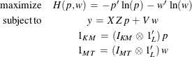
where
![\[ \beta \: = \: Z \, p \]](images/etsug_entropy0082.png)
![\[ \! \! \! \! \! \! \! \! \! \! \! \! \! \! \! \! \ \! \! \! \! \! \! \! \! \! \! \! \! \! \! \! \! \! \! \! \! \! \! \! \! Z \: = \: \left[ \begin{array}{ccccccccccccccc} z_{11}^{1} & \cdot \cdot \cdot & z_{L1}^{1} & 0 & 0 & 0 & 0 & 0 & 0 & 0 & 0 & 0 & 0 & 0 & 0 \\ 0 & 0 & 0 & \ddots & 0 & 0 & 0 & 0 & 0 & 0 & 0 & 0 & 0 & 0 & 0 \\ 0 & 0 & 0 & 0 & z_{11}^{K} & \cdot \cdot \cdot & z_{L1}^{K} & 0 & 0 & 0 & 0 & 0 & 0 & 0 & 0 \\ 0 & 0 & 0 & 0 & 0 & 0 & 0 & \ddots & 0 & 0 & 0 & 0 & 0 & 0 & 0 \\ 0 & 0 & 0 & 0 & 0 & 0 & 0 & 0 & z_{1M}^{1} & \cdot \cdot \cdot & z_{LM}^{1} & 0 & 0 & 0 & 0 \\ 0 & 0 & 0 & 0 & 0 & 0 & 0 & 0 & 0 & 0 & 0 & \ddots & 0 & 0 & 0 \\ 0 & 0 & 0 & 0 & 0 & 0 & 0 & 0 & 0 & 0 & 0 & 0 & z_{1M}^{K} & \cdot \cdot \cdot & z_{LM}^{K} \end{array} \right] \]](images/etsug_entropy0083.png)
![\[ p \: = \: \left[ \begin{array}{ccccccccccccccc} p_{11}^{1} & \cdot & p_{L1}^{1} & \cdot & p_{11}^{K} & \cdot & p_{L1}^{K} & \cdot & p_{1M}^{1} & \cdot & p_{LM}^{1} & \cdot & p_{1M}^{K} & \cdot & p_{LM}^{K} \end{array} \right]’ \]](images/etsug_entropy0084.png)
![\[ e \: = \: V \, w \]](images/etsug_entropy0085.png)
![\[ \! \! \! \! \! \! \! \! \! \! \! \! \! \! \! \! \ \! \! \! \! \! \! \! \! \! \! \! \! \! \! \! \! \! \! \! \! \! \! \! \! V \: = \: \left[ \begin{array}{ccccccccccccccc} v_{11}^{1} & \cdot \cdot \cdot & v_{11}^{L} & 0 & 0 & 0 & 0 & 0 & 0 & 0 & 0 & 0 & 0 & 0 & 0 \\ 0 & 0 & 0 & \ddots & 0 & 0 & 0 & 0 & 0 & 0 & 0 & 0 & 0 & 0 & 0 \\ 0 & 0 & 0 & 0 & v_{1T}^{1} & \cdot \cdot \cdot & v_{1T}^{L} & 0 & 0 & 0 & 0 & 0 & 0 & 0 & 0 \\ 0 & 0 & 0 & 0 & 0 & 0 & 0 & \ddots & 0 & 0 & 0 & 0 & 0 & 0 & 0 \\ 0 & 0 & 0 & 0 & 0 & 0 & 0 & 0 & v_{M1}^{1} & \cdot \cdot \cdot & v_{M1}^{L} & 0 & 0 & 0 & 0 \\ 0 & 0 & 0 & 0 & 0 & 0 & 0 & 0 & 0 & 0 & 0 & \ddots & 0 & 0 & 0 \\ 0 & 0 & 0 & 0 & 0 & 0 & 0 & 0 & 0 & 0 & 0 & 0 & v_{MT}^{1} & \cdot \cdot \cdot & v_{MT}^{L} \end{array} \right] \]](images/etsug_entropy0086.png)
![\[ \! \! \! \! \! \! \! \! \! \! w \: = \: \left[ \begin{array}{ccccccccccccccc} w_{11}^{1} & \cdot & w_{11}^{L} & \cdot & w_{1T}^{1} & \cdot & w_{1T}^{L} & \cdot & w_{M1}^{1} & \cdot & w_{M1}^{L} & \cdot & w_{MT}^{1} & \cdot & w_{MT}^{L} \end{array} \right]’ \, \]](images/etsug_entropy0087.png)
y denotes the MT column vector of observations of the dependent variables;  denotes the (MT x KM ) matrix of observations for the independent variables; p denotes the LKM column vector of weights associated with the points in Z; w denotes the LMT column vector of weights associated with the points in V;
  ,
,  , and
, and  are L-, KM-, and MT-dimensional column vectors, respectively, of ones; and
  and
and  are (KM x KM) and (MT x MT) dimensional identity matrices. The subscript l denotes the support point
  , k denotes the parameter
  , m denotes the equation
 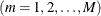 , and t denotes the observation
  .
.
Using this notation, the maximum entropy problem that is analogous to the OLS problem used as the initial step of the traditional SUR approach is
The results are GME-SUR estimates with independent errors, the analog of OLS. The covariance matrix  is computed based on the residual of the equations,
  . An
. An  factorization of the is used to compute the square root of the matrix.
After solving this problem, these entropy-based estimates are analogous to the Aitken two-step estimator. For iterative GME-SUR,
the covariance matrix of the errors is recomputed, and a new is computed and factored. As in traditional ITSUR, this process repeats until the covariance matrix and the parameter estimates
converge.
The estimation of the parameters for the normed-moment version of SUR (GME-SUR-NM) uses an identical process. The constraints for GME-SUR-NM is defined as:
![\[ X’y \: = \: X’(\mb{S} ^{-1} {\otimes } \mb{I} )X \, Z \, p \: + \: X’(\mb{S} ^{-1} {\otimes } \mb{I} )V \, w \]](images/etsug_entropy0100.png)
The estimation of the parameters for GME-SUR-NM uses an identical process as outlined previously for GME-SUR.