The AUTOREG Procedure

Many time series exhibit high positive autocorrelation, having the smooth appearance of a random walk. This behavior can be explained by the partial adjustment and adaptive expectation hypotheses.

Short-term forecasting applications often use autoregressive models because these models absorb the behavior of this kind of data. In the case of a first-order AR process where the autoregressive parameter is exactly 1 (a random walk ), the best prediction of the future is the immediate past.

PROC AUTOREG can often greatly improve the fit of models, not only by adding additional parameters but also by capturing the random walk tendencies. Thus, PROC AUTOREG can be expected to provide good short-term forecast predictions.

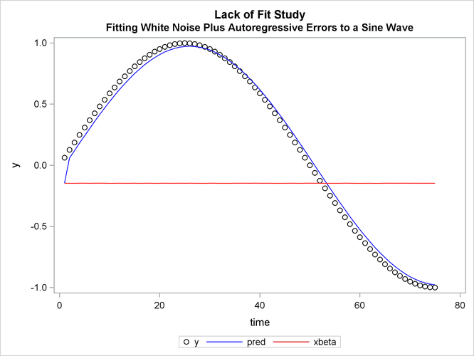
However, good forecasts do not necessarily mean that your structural model contributes anything worthwhile to the fit. In the following example, random noise is fit to part of a sine wave. Notice that the structural model does not fit at all, but the autoregressive process does quite well and is very nearly a first difference (AR(1) = ). The DATA step, PROC AUTOREG step, and PROC SGPLOT step follow:

title1 'Lack of Fit Study';
title2 'Fitting White Noise Plus Autoregressive Errors to a Sine Wave';

data a;
   pi=3.14159;
   do time = 1 to 75;
      if time > 75 then y = .;
      else y = sin( pi * ( time / 50 ) );
      x = ranuni( 1234567 );
      output;
   end;
run;

proc autoreg data=a plots;
   model y = x / nlag=1;
   output out=b p=pred pm=xbeta;
run;

proc sgplot data=b;
   scatter y=y x=time / markerattrs=(color=black);
   series y=pred x=time / lineattrs=(color=blue);
   series y=xbeta x=time / lineattrs=(color=red);
run;

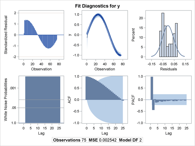
The printed output produced by PROC AUTOREG is shown in Output 9.3.1 and Output 9.3.2. Plots of observed and predicted values are shown in Output 9.3.3 and Output 9.3.4. Note: the plot Output 9.3.3 can be viewed in the Autoreg.Model.FitDiagnosticPlots category by selecting View→Results.

Output 9.3.3: Diagnostics Plots

Output 9.3.4: Plot of Autoregressive Prediction