The COPULA Procedure (Experimental)
- Overview
- Getting Started
-
Syntax

-
Details
Sklar’s Theorem Dependence Measures Normal Copula Student’s t copula Archimedean Copulas Canonical Maximum Likelihood Estimation (CMLE) Exact Maximum Likelihood Estimation (MLE) Calibration Estimation Nonlinear Optimization Options Displayed Output OUTCOPULA= Data Set OUTPSEUDO=, OUT=, and OUTUNIFORM= Data Sets ODS Table Names ODS Graph Names
-
Examples
- References
Example 10.1 Copula Based VaR Estimation
Value-at-risk (VaR) has become a de facto standard in financial risk management. The purpose of this measure is to give some quantitative insight to the riskiness of an asset portfolio. This measure is expressed generically in the following terms: What is the probability of losing no more than given percentage of a portfolio in a certain period of time? Or, what are the maximum possible losses at a given confidence level? The most simple and clearly wrong answer to this question is to compute the empirical quantile of past portfolio returns. The problem of this approach is that it does not take into account the dynamic nature of asset returns, the possibility of changing distribution, time memory, and, most importantly, cross-sectional dependence between individual assets in the portfolio.
This simple example of VaR computation takes into account at least cross-sectional dependence of the data. The end result is the prediction of the next-day maximum possible loss on the portfolio of stocks.
This example uses the daily returns on large stocks such as IBM, Microsoft, British Petroleum, Coca Cola, and Duke Energy. Output 10.1.1 shows the first 10 observations of the data.
| Obs | date | ret_msft | ret_ko | ret_ibm | ret_duk | ret_bp |
|---|---|---|---|---|---|---|
| 1 | 01/03/2008 | 0.004182 | 0.010367 | 0.002002 | 0.003503 | 0.019114 |
| 2 | 01/04/2008 | -0.027960 | 0.001913 | -0.035861 | -0.000582 | -0.014536 |
| 3 | 01/07/2008 | 0.006732 | 0.023607 | -0.010671 | 0.025611 | 0.017922 |
| 4 | 01/08/2008 | -0.033435 | 0.004239 | -0.024610 | -0.002838 | -0.016049 |
| 5 | 01/09/2008 | 0.029560 | 0.026680 | 0.007301 | 0.010814 | -0.027078 |
| 6 | 01/10/2008 | -0.003054 | 0.004441 | 0.016414 | -0.001689 | -0.004395 |
| 7 | 01/11/2008 | -0.012255 | -0.027346 | -0.022546 | -0.012408 | -0.018473 |
| 8 | 01/14/2008 | 0.013958 | 0.008418 | 0.053857 | 0.003427 | 0.001166 |
| 9 | 01/15/2008 | -0.011318 | -0.010851 | -0.010689 | -0.017075 | -0.040925 |
| 10 | 01/16/2008 | -0.022587 | -0.015021 | -0.001955 | 0.002316 | -0.021336 |
The purpose of this exercise is to estimate one-day future losses of a stock portfolio. The simplest approach is to assume that the joint distribution of individual asset returns does not change with time. This might be close to the truth if only a small time interval is used. Then, a copula approach is used to estimate the joint distribution. Next, the new large sample of daily individual asset returns is simulated from the fitted joint distribution. These assets are then combined into a portfolio and its daily returns are computed. Finally, quantiles of simulated portfolio returns (which simply represent possible next-day losses of the portfolio) are examined.
So, the first step is to cut off a small number of past return observations as in the following SAS data step:
/* Keep only the last 250 observations of the data */
data returns;
   set returns nobs=observ;
   if (_N_ > observ-250);
run;
The following statements fit a  copula to the returns data and at the same time simulate the sample from the fitted joint distribution:
/* Copula estimation and simulation of returns */
proc copula data = returns;
   var ret_ibm ret_msft ret_bp ret_ko ret_duk;
   * fit T-copula to stock returns;
   fit T /
          marginals = empirical
          method    = MLE
          plots      = (data = both matrix);
   * simulate 10000 observations;
   * independent in time, dependent in cross-section;
   simulate /
            ndraws = 10000
            seed   = 1234
            out    = simulated_returns
            plots = (data = original scatter);
run;
The first line of COPULA procedure uses a VAR statement to specify the list of variables. In this example, these are daily returns of five large-company stocks.The next statement, FIT, requires some options. First, Student’s copula (T) is specified. After the slash, the MARGINALS=EMPIRICAL option specifies that an empirical distribution be fit. The choice of fitting method is MLE. The PLOTS=BOTH MATRIX option requests that both original and transformed data graphs be organized into a symmetric panel.
Then, given the estimation results, the NDRAWS= option in the SIMULATE statement simulates 10,000 new observations for each asset return series. The SEED= option fixes the random number generator, the OUT= option specifies the name of SAS data set to contain the simulated sample, and the PLOT= option requests scatter plots of simulated returns in the original data scale.
The output of these statements is shown in Output 10.1.2.
| Model Fit Summary | |
|---|---|
| Number of Observations | 250 |
| Data Set | WORK.RETURNS |
| Model | T |
| Log Likelihood | 171.52064 |
| Maximum Absolute Gradient | 7.91523E-7 |
| Number of Iterations | 9 |
| Optimization Method | Newton-Raphson |
| AIC | -321.04128 |
| SBC | -282.30521 |
| Parameter Estimates | ||||
|---|---|---|---|---|
| Parameter | Estimate | Standard Error | t Value | Approx Pr > |t| |
| DF | 6.714101 | 1.338752 | 5.02 | <.0001 |
| Correlation Matrix | |||||
|---|---|---|---|---|---|
| ret_ibm | ret_msft | ret_bp | ret_ko | ret_duk | |
| ret_ibm | 1.000000000 | 0.565737845 | 0.466209147 | 0.454771683 | 0.474020099 |
| ret_msft | 0.565737845 | 1.000000000 | 0.458469772 | 0.323355456 | 0.365773073 |
| ret_bp | 0.466209147 | 0.458469772 | 1.000000000 | 0.345866479 | 0.357634010 |
| ret_ko | 0.454771683 | 0.323355456 | 0.345866479 | 1.000000000 | 0.474150256 |
| ret_duk | 0.474020099 | 0.365773073 | 0.357634010 | 0.474150256 | 1.000000000 |
The first table in Output 10.1.2, “Model Fit Summary,” provides some general description of copula model estimation. The second table, “Parameter Estimates,” provides point estimates and inference on copula parameters. In this example the only parameter in this table is the number of degrees of freedom in the multivariate distribution. The last table, “Correlation Matrix,” contains estimates of copula model parameters.
The graphical output of the preceding statements is in Output 10.1.3 and in Output 10.1.4.
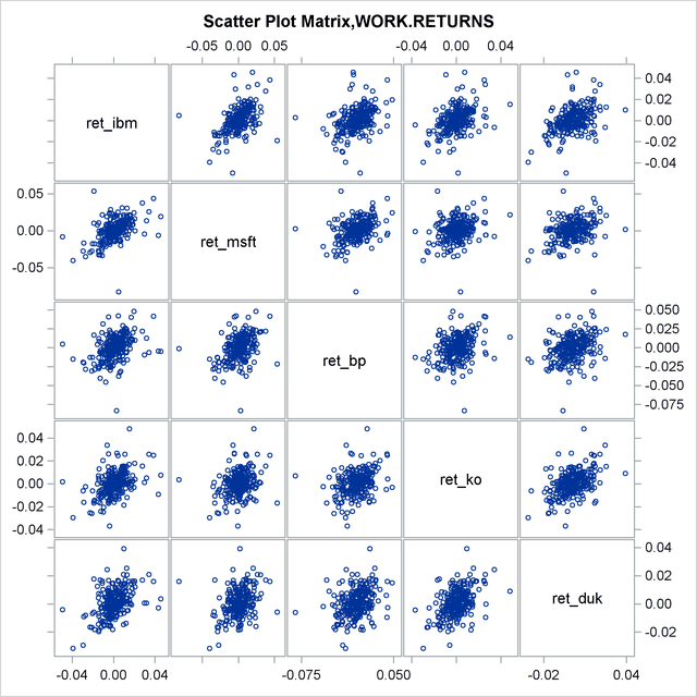
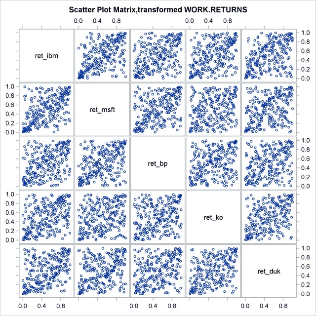
Note that in Output 10.1.3 the most elliptical scatter plot, between IBM and MSFT, indicates the strongest dependence. Similarly, in Output 10.1.4 those graphs that are denser along the diagonal indicate the same thing.
Now the equally weighted next day portfolio return is computed. Each individual return is transformed into nominal scale first, then all returns are added up with equal weights, and the result is transformed into a net return by subtracting one.
/* compute equally weighted portfolio return */
data port_ret (drop = i ret);
   set simulated_returns;
   array returns{5} ret_ibm ret_msft ret_bp ret_ko ret_duk;
   ret =0;
   do i =1 to 5;
      ret = ret+ 0.2*exp(returns[i]);
   end;
   port_ret = ret-1;
run;
The final step is to compute empirical quantiles of simulated daily portfolio return. This is done with the help of PROC UNIVARIATE in the following statements:
/* compute descriptive statistics */
/* quantile table will give Value-at-Risk estimates for the portfolio */
proc univariate data = port_ret;
   var port_ret;
run;
Output 10.1.5 shows that with 99% confidence the potential loss on an equally weighted portfolio over the next day does not exceed 2.7% (the number in table is multiplied by 100). You can also say that there is no more than 5% chance of losing 1.5% of the portfolio value. These percentage measures are exactly the value-at-risk.
| Quantiles (Definition 5) | |
|---|---|
| Quantile | Estimate |
| 100% Max | 0.048144752 |
| 99% | 0.026628900 |
| 95% | 0.015538138 |
| 90% | 0.011573970 |
| 75% Q3 | 0.005799792 |
| 50% Median | 0.000688678 |
| 25% Q1 | -0.004953853 |
| 10% | -0.010637126 |
| 5% | -0.014677418 |
| 1% | -0.026631117 |
| 0% Min | -0.052757715 |