The COPULA Procedure (Experimental)

Simulation

The input parameters for the simulation are . The copula can be simulated by the following the two steps:

1. Generate a multivariate vector following the centered t distribution with degrees of freedom and correlation matrix .

2. Transform the vector into 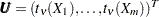, where is the distribution function of univariate t distribution with degrees of freedom.

To simulate centered multivariate t random variables, you can use the property that if , where and the univariate random variable .

Fitting

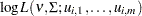
To fit a copula is to estimate the covariance matrix anddegrees of freedom from a given multivariate data set. Given a random sample, that has uniform marginal distributions, the log likelihood is

where denotes the degrees of freedom of the t copula, denotes the joint density function of the centered multivariate t distribution with parameters , is the distribution function of a univariate t distribution with degrees of freedom, is a correlation matrix, and is the density function of univariate t distribution with degrees of freedom.

The log likelihood can be maximized with respect to the parameters using numerical optimization. If you allow the parameters in to be such that is symmetric and with ones on the diagonal, then the MLE estimate for might not be positive semidefinite. In that case, you need to apply the adjustment to convert the estimated matrix to positive semidefinite, as shown by McNeil, Frey, and Embrechts (2005), Algorithm 5.55.

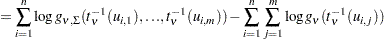
When the dimension of the data increases, the numerical optimization quickly becomes infeasible. It is common practice to estimate the correlation matrix by calibration using Kendall’s tau. Then, using this fixed , the single parameter can be estimated by MLE. By proposition 5.37 in McNeil, Frey, and Embrechts (2005),

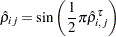
where is the Kendall’s tau and is the off-diagonal elements of the correlation matrix of the t copula. Therefore, an estimate for the correlation is

where and are the estimates of the sample correlation matrix and Kendall’s tau, respectively. However, it is possible that the estimate of the correlation matrix is not positive definite. In this case, there is a standard procedure that uses the eigenvalue decomposition to transform the correlation matrix into one that is positive definite. Let be a symmetric matrix with ones on the diagonal, with off-diagonal entries in . If is not positive semidefinite, use Algorithm 5.55 from McNeil, Frey, and Embrechts (2005):

1. Compute the eigenvalue decomposition , where is a diagonal matrix that contains all the eigenvalues and is an orthogonal matrix that contains the eigenvectors.

2. Construct a diagonal matrix by replacing all negative eigenvalues in by a small value .

3. Compute , which is positive definite but not necessarily a correlation matrix.

4. Apply the normalizing operator on the matrix to obtain the correlation matrix desired.

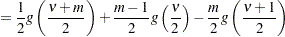
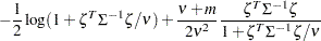
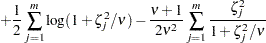
The log likelihood function and its gradient function for a single observation are listed as follows, where , with , and is the derivative of the function:

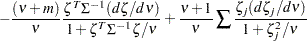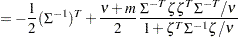
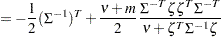
The derivative of the likelihood with respect to the correlation matrix follows: