The COPULA Procedure (Experimental)

Overview of Archimedean Copulas

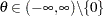
Let function 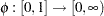be a strict Archimedean copula generator function and suppose its inverse is completely monotonic on . A strict generator is a decreasing function that satisfies and . A decreasing function 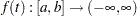is completely monotonic if it satisfies

An Archimedean copula is defined as follows:

The Archimedean copulas available in the COPULA procedure are the Clayton copula, the Frank copula, and the Gumbel copula.

Clayton Copula

Let the generator function . A Clayton copula is defined as

with .

Frank Copula

Let the generator function be

A Frank copula is defined as

with for and for .

Gumbel Copula

Let the generator function . A Gumbel copula is defined as

with .

Simulation

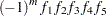
Suppose the generator of the Archimedean copula is . Then the simulation method using Laplace-Stieltjes transformation of the distribution function is given by Marshall and Olkin (1988) where :

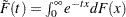1. Generate a random variable with the distribution function such that .

2. Draw samples from independent uniform random variables .

3. Return .

The Laplace-Stieltjes transformations are as follows:

• For the Clayton copula, , and the distribution function is associated with a Gamma random variable with shape parameter and scale parameter one.

• For the Gumbel copula, , and is the distribution function of the stable variable with .

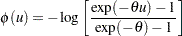
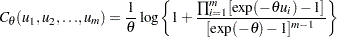
• For the Frank copula with , , and is a discrete probability function . This probability function is related to a logarithmic random variable with parameter value .

For details about simulating a random variable from a stable distribution, see Theorem 1.19 in Nolan (2010). For details about simulating a random variable from a logarithmic series, see Chapter 10.5 in Devroye (1986).

For a Frank copula with and , the simulation can be done through conditional distributions as follows:

1. Draw independent from a uniform distribution.

2. Let .

3. Let .

Fitting

One method to estimate the parameters is to calibrate with Kendall’s tau. The relation between the parameter and Kendall’s tau is summarized in the following table for the three Archimedean copulas.

Table 10.2 Calibration Using Kendall’s Tau

Copula Type		Formula for
Clayton
Gumbel
Frank		No closed form

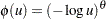
In Table 10.2, for , and for . In addition, for the Frank copula, the formula for has no closed form. The numerical algorithm for root finding can be used to invert the function to obtain as a function of .

Alternatively, you can use the MLE or the CMLE method to estimate the parameter given the data and . The log-likelihood function for each type of Archimedean copula is provided in the following sections.

Fitting the Clayton Copula
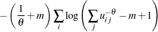
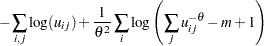
For the Clayton copula, the log-likelihood function is as follows (Cherubini, Luciano and Vecchiato 2004, Chapter 7):

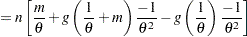
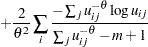
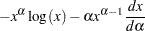
Let be the derivative of . Then the first order derivative is

The second order derivative is

Fitting the Gumbel Copula

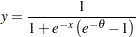
A different parameterization is used for the following part, which is related to the fitting of the Gumbel copula. For Gumbel copula, you need to compute . It turns out that for ,

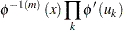
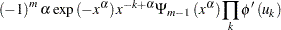
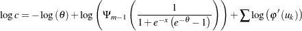
where is a function that is described later. The copula density is given by

where , , ,,, and .

The log density is

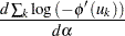
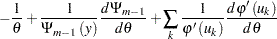
Now the first order derivative of the log density has the decomposition

Some of the terms are given by

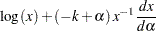where

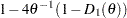
The last term in the derivative of the is

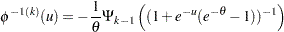
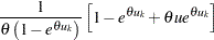
Now the only remaining term is , which is related to . Wu, Valdez, and Sherris (2007) show that satisfies a recursive equation

with .

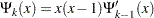
The preceding equation implies that is a polynomial of and therefore can be represented as

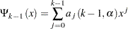In addition, its coefficient, denoted by , is a polynomial of . For simplicity, use the notation 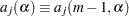. Therefore,

Fitting the Frank copula

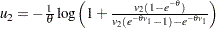
For the Frank copula,

When , a Frank copula has a probability density function

where .

The log likelihood is

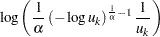
Denote

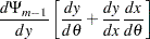
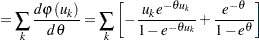
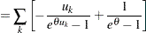
Then the derivative of the log likelihood is

The term in the last summation is

The function satisfies a recursive relation

with . Note that is a polynomial whose coefficients do not depend on ; therefore,

where

For the case of and , the bivariate density is