Usage Note 70062: Modeling the mean and variance for a normal response and testing effects on both
 |  |  |
Regression and analysis of variance models for normally-distributed responses assume that the variance is constant (homogeneous) across the populations in the data. The populations are defined as the unique combinations of settings of the predictor variables in the model. To obtain good estimates of the effects on the mean, it is important for the model to adjust for any variance differences among the populations. Additionally, it might be of interest to estimate the effects of variables on the variance and to test hypotheses about functions of those effects.
For the simple one-way ANOVA model that contains a single CLASS predictor, tests for equal variance are available using the HOVTEST= option in the GLM procedure. If variances are found to be unequal, Welch's test is available to test equality of the means. See the example titled "Testing for Equal Group Variances" in the PROC GLM documentation. However, as noted in the GLM documentation, the regression and ANOVA model is fairly robust to some departure from variance equality and the statistical power of the HOVTEST tests might not be sufficient to indicate the need for alternative analysis.
In more complex models, if one or more categorical variables define populations that can exhibit differing variance, the GLIMMIX procedure can be used to estimate the population variances and provide a test of their equality. In models with multiple predictors, some combination of them, possibly including continuous predictors, might affect the variance significantly. For these situations, as well as those described above, it is useful to have a flexible modeling approach that allows you to model both the mean and the variance using separate functions of available predictor variables. This approach also allows you to adjust the mean model for differing variance, test for significant effects on the variance, and estimate and test linear or nonlinear functions of the effects on the variance such as variance ratios. With the NLMIXED and QLIM procedures, you can specify separate models for the mean and variance. The following examples illustrate the use of the procedures and methods discussed above.
Example 1: Normal Data with Known Means and Variances
The following DATA step generates a data set for two processes, P, producing a normally distributed response, Y, at each of several levels of a covariate, X, for X=10, 11, ... , 15. For process A, the mean is equal to X and for process B, the mean equals 3X. Also, the variance for process A is 4 while it is 25 for process B. The true mean model can then be written as follows:
E(Y) = ba*pa*x + bb*pb*x , where pa=1 if p="a", 0 otherwise (similarly for pb) and where the mean model parameters are ba=1 and bb=3.
and, assuming a log-linear form of the model for the variance,
log(V(Y)) = log(va)*pa + log(vb)*pb , where the log variance model parameters are va=4 and vb=25.
Note that the variance ratio, va/vb = 4/25 = 0.16. Also note that the process intercepts are both zero (the means equal zero when X=0), but the process slopes are 1 and 3.
     data semi;
        drop j;
        call streaminit(4252);
        do p = 'a','b';
          p1=(p='a');
          do x = 10 to 15;
             do j = 1 to 100;
                mean = (p="a")*x + (p="b")*3*x;
                logvar = (p="a")*log(4) + (p="b")*log(25);
                y = rand("normal",mean,sqrt(exp(logvar)));
                output;
             end;
          end;
        end;
        run;
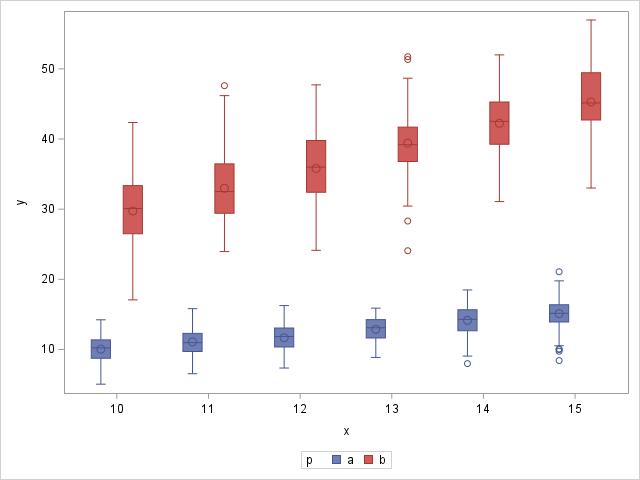
The following statements produce box plots that show the changing means and variances as well as their values in the data:
     proc sort data=semi;
        by x;
        run;
     proc sgplot;
        vbox y / category=x group=p;
        run;
     proc means n mean std var;
        class p x; var y;
        run;
Note the difference in variability in the box plots for processes A and B.
 |
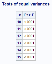
Since the model for these data involves X as a covariate in addition to P, it is not a one-way model. However, as mentioned in SAS Note 22526, the variance test available in PROC GLM with the HOVTEST= option can be used by fitting the one-way model at each level of X. The following does that and summarizes the results of the Levene test for equal variances in each level of X:
     ods exclude all;
        proc glm data=semi; by x;
           class p;
           model y = p;
           means p / hovtest=levene;
           ods output hovftest=lev(where=(probf>0) keep=x probf);
           quit;
     ods select all;
     proc print label;
        id x; var probf;
        title "Tests of equal variances";
        run;
The results show clear evidence of unequal variances in each level of X:
 |
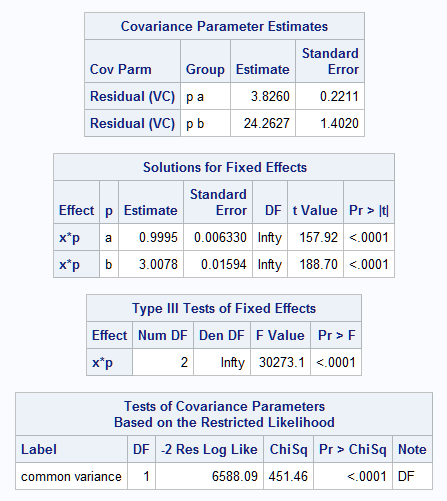
PROC GLIMMIX (and PROC MIXED as mentioned in SAS Note 22526) can also be used to fit the mean model while allowing for the processes to have differing variance. The following statements fit the mean model described above that has zero intercepts and different slopes for the processes (see SAS Note 24177 on a general approach to test for differing group slopes). The DDFM=NONE option creates large-sample tests. The RANDOM statement using the GROUP= option estimates separate variances for the processes. The COVTEST statement provides a test of variance equality. However, the effect of X as a continuous effect on the variance cannot be assessed.
     proc glimmix data=semi;
        class p;
        model y=p*x / noint solution ddfm=none;
        random _residual_ / group=p;
        covtest 'common variance' homogeneity;
        run;
The results show that the true mean model and the two process variances are well estimated. The null hypothesis of variance equality is rejected (p<0.0001).
 |
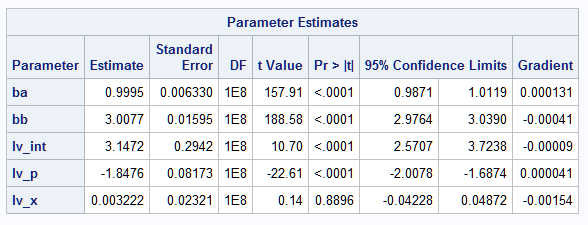
PROC NLMIXED is used below to fit separate mean and variance models. The log variance model includes parameters for the effect of the categorical process predictor as well as the linear effect of X, where X is treated as a continuous variable as it is in the mean model. In the model, (p="a") creates a 0,1-coded dummy variable for process A. Its parameter in the variance model, lv_p, estimates the difference in the effect of the two processes in the same way that a parameter of a CLASS variable is interpreted in other procedures. The DF=1e8 option creates tests that are large-sample tests and confidence intervals:
     proc nlmixed data=semi df=1e8;
        mean=ba*(p="a")*x + bb*(p="b")*x;
        logvar=lv_int + lv_p*(p="a") + lv_x*x;
        var=exp(logvar);
        model y ~ normal(mean,var);
        run;
Note that process, P, has a significant effect on the log variance, but X does not. This suggests that the variances are unequal among the populations and that the inequality is due to the different processes.
 |
An equivalent model can now be fit that reparameterizes the log variance model to more directly estimate the variances in the two processes. The ESTIMATE statements provide an estimate of the ratio of the variances as well as test if their ratio is equal to one:
     proc nlmixed data=semi df=1e8;
        mean=ba*(p="a")*x + bb*(p="b")*x;
        logvar=log(va)*(p="a") + log(vb)*(p="b");
        var=exp(logvar);
        model y ~ normal(mean,var);
        estimate 'Estimate var ratio' va/vb;
        estimate 'Test var ratio=1' 1-va/vb;
        run;
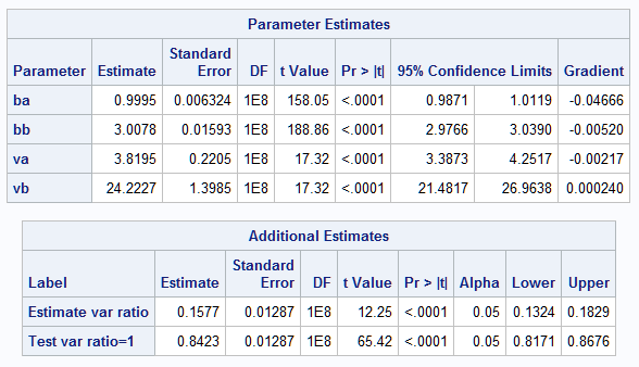
This final model closely estimates the parameters of the true mean and variance models. The results essentially match those from the GLIMMIX model above. The estimate of the variance ratio, 0.1577, also closely approximates the true variance ratio, 0.16. The test that the ratio equals one, meaning equal variances, is clearly rejected (p<0.0001). Note that in the previous parameterization of the model, the process parameter estimate, lv_p = -1.8465, is the difference in the log variances of the two processes. So, the variance ratio can also be obtained from it as exp(-1.8476) = 0.1576.
 |
Modeling both the mean and variance can also be achieved using the QLIM procedure in SAS/ETS®. The mean model is specified in the MODEL statement and the variance model is specified in the HETERO statement. The LINK=EXP and NOCONST options produce the equivalent variance model as described above, though the intercept is parameterized differently. The results are essentially the same as from the first NLMIXED model above. The DATA step estimates the variance ratio and a 95% large-sample confidence interval:
     proc qlim data=semi;
        class p;
        model y = p*x / noint;
        hetero y ~ p1 x / link=exp noconst;
        ods output parameterestimates=pe(where=(parameter="_H.p1"));
        run;
     data pe; set pe;
        VarRatio=exp(estimate);
        LCL=exp(estimate-probit(.975)*stderr);
        UCL=exp(estimate+probit(.975)*stderr);
        run;
     proc print data=pe noobs;
        var VarRatio LCL UCL;
        run;
Example 2: Multiple Predictors
The following example uses data from a designed experiment in which shrinkage is measured at settings of several predictors. These statements create the data set for analysis:
     data bt;
       input
       SHRINK    TIME    MTEMP     THICK     HPRESS     SPEED     HTIME     GATE;
       datalines;
       2.2       -1       -1        -1         -1        -1        -1        -1
       2.1       -1       -1        -1         -1        -1        -1        -1
       2.3       -1       -1        -1         -1        -1        -1        -1
       2.3       -1       -1        -1         -1        -1        -1        -1
       0.3       -1       -1        -1          1         1         1         1
       2.5       -1       -1        -1          1         1         1         1
       2.7       -1       -1        -1          1         1         1         1
       0.3       -1       -1        -1          1         1         1         1
       0.5       -1        1         1         -1        -1         1         1
       3.1       -1        1         1         -1        -1         1         1
       0.4       -1        1         1         -1        -1         1         1
       2.8       -1        1         1         -1        -1         1         1
         2       -1        1         1          1         1        -1        -1
       1.9       -1        1         1          1         1        -1        -1
       1.8       -1        1         1          1         1        -1        -1
         2       -1        1         1          1         1        -1        -1
         3        1       -1         1         -1         1        -1         1
       3.1        1       -1         1         -1         1        -1         1
         3        1       -1         1         -1         1        -1         1
         3        1       -1         1         -1         1        -1         1
       2.1        1       -1         1          1        -1         1        -1
       4.2        1       -1         1          1        -1         1        -1
         1        1       -1         1          1        -1         1        -1
       3.1        1       -1         1          1        -1         1        -1
         4        1        1        -1         -1         1         1        -1
       1.9        1        1        -1         -1         1         1        -1
       4.6        1        1        -1         -1         1         1        -1
       2.2        1        1        -1         -1         1         1        -1
         2        1        1        -1          1        -1        -1         1
       1.9        1        1        -1          1        -1        -1         1
       1.9        1        1        -1          1        -1        -1         1
       1.8        1        1        -1          1        -1        -1         1
     ;
To investigate the possibility that some of the variables might be factors influencing the response variance as well as its mean, the following model is fit. It includes a main effects model both for the mean and for the log variance:
     proc nlmixed data=bt df=1e8;
        mean=int + b1*time + b2*mtemp + b3*thick + b4*hpress + b5*speed + b6*htime + b7*gate;
        logvar=lv_int + lv_time*time + lv_m*mtemp + lv_th*thick + lv_hp*hpress + lv_s*speed +
               lv_ht*htime + lv_g*gate;
        var=exp(logvar);
        model shrink ~ normal(mean,var);
        run;
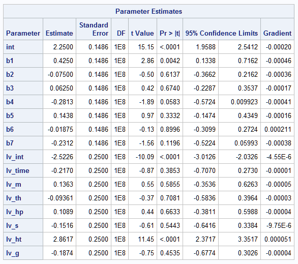
For the mean, only the parameters for TIME and HPRESS (b1 and b4) are at least marginally significant. There is strong evidence that HTIME has an effect on the log variance.
 |
Given the above results, the following statements fit a simplified model that includes just the predictors found to be significant. The log variance model is reparameterized to estimate the log variance estimates at the two levels of HTIME and the variance ratio. A test that the variance ratio equals one is also provided:
     proc nlmixed data=bt df=1e8;
        mean=int + b1*time + b4*hpress;
        logvar=log(v6hi)*(htime=1) + log(v6lo)*(htime=-1);
        var=exp(logvar);
        model shrink ~ normal(mean,var);
        estimate 'Estimate var ratio' v6hi/v6lo;
        estimate 'Test var ratio=1' v6hi/v6lo-1;
        run;
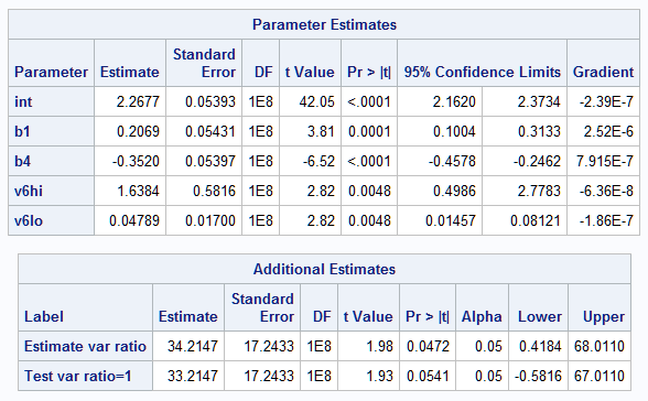
The results show a marginally significant effect on the variance (p=0.0541) with variance ratio equal to 34.2. The estimated variance at HTIME=1 is 1.638 but only 0.048 at HTIME=-1.
 |
As noted above, the regression and ANOVA model is fairly robust to departures from the usual assumptions. So, it is interesting to compare the above results to those from the homogeneous variance model to see the effect that adjusting for differing variance has on conclusions about the effects on the mean. The NLMIXED step below fits the same mean model as above but estimates only a common variance. PROC GENMOD (and other procedures) can also fit the model as shown (though GENMOD estimates the common standard deviation rather than the variance):
    proc nlmixed data=bt df=1e8;
        mean=int + b1*time + b4*hpress;
        model shrink ~ normal(mean,var);
        run;
    proc genmod data=bt;
        model shrink=time hpress;
        run;
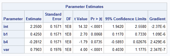
Below are the results from the NLMIXED model. Note the larger standard errors and p-values for the mean model parameters in the homogeneous variance model as compared to the heterogeneous variance model above. Adjusting for differing variance with the heterogeneous variance model allowed the effect of HPRESS to become significant (p<0.0001) but not in the homogeneous variance model (p=0.0735).
 |
Operating System and Release Information
| Product Family | Product | System | SAS Release | |
| Reported | Fixed* | |||
| SAS System | SAS/STAT | OpenVMS Alpha | ||
| Linux on Itanium | ||||
| Linux for x64 | ||||
| Linux | ||||
| IRIX | ||||
| HP-UX IPF | ||||
| HP-UX | ||||
| AIX | ||||
| ABI+ for Intel Architecture | ||||
| 64-bit Enabled Solaris | ||||
| 64-bit Enabled HP-UX | ||||
| 64-bit Enabled AIX | ||||
| Windows Vista for x64 | ||||
| Windows Vista | ||||
| Windows Millennium Edition (Me) | ||||
| Windows 7 Ultimate x64 | ||||
| Windows 7 Ultimate 32 bit | ||||
| Windows 7 Professional x64 | ||||
| Windows 7 Professional 32 bit | ||||
| Windows 7 Home Premium x64 | ||||
| Windows 7 Home Premium 32 bit | ||||
| Windows 7 Enterprise x64 | ||||
| Windows 7 Enterprise 32 bit | ||||
| Microsoft Windows XP Professional | ||||
| Microsoft Windows Server 2022 | ||||
| Microsoft Windows Server 2019 | ||||
| Microsoft Windows Server 2016 | ||||
| Microsoft Windows Server 2012 Std | ||||
| Microsoft Windows Server 2012 R2 Std | ||||
| Microsoft Windows Server 2012 R2 Datacenter | ||||
| Microsoft Windows Server 2012 Datacenter | ||||
| Microsoft Windows Server 2008 for x64 | ||||
| Microsoft Windows Server 2008 R2 | ||||
| Microsoft Windows Server 2008 | ||||
| Microsoft Windows Server 2003 for x64 | ||||
| Microsoft Windows Server 2003 Standard Edition | ||||
| Microsoft Windows Server 2003 Enterprise Edition | ||||
| Microsoft Windows Server 2003 Datacenter Edition | ||||
| Microsoft Windows NT Workstation | ||||
| Microsoft Windows 2000 Professional | ||||
| Microsoft Windows 2000 Server | ||||
| Microsoft Windows 2000 Datacenter Server | ||||
| Microsoft Windows 2000 Advanced Server | ||||
| Microsoft Windows 95/98 | ||||
| Microsoft Windows 11 | ||||
| Microsoft Windows 10 | ||||
| Microsoft Windows 8.1 Pro x64 | ||||
| Microsoft Windows 8.1 Pro 32-bit | ||||
| Microsoft Windows 8.1 Enterprise x64 | ||||
| Microsoft Windows 8.1 Enterprise 32-bit | ||||
| Microsoft Windows 8 Pro x64 | ||||
| Microsoft Windows 8 Pro 32-bit | ||||
| Microsoft Windows 8 Enterprise x64 | ||||
| Microsoft Windows 8 Enterprise 32-bit | ||||
| OS/2 | ||||
| Microsoft® Windows® for x64 | ||||
| Microsoft Windows XP 64-bit Edition | ||||
| Microsoft Windows Server 2003 Enterprise 64-bit Edition | ||||
| Microsoft Windows Server 2003 Datacenter 64-bit Edition | ||||
| Microsoft® Windows® for 64-Bit Itanium-based Systems | ||||
| OpenVMS VAX | ||||
| z/OS 64-bit | ||||
| z/OS | ||||
| OpenVMS on HP Integrity | ||||
| Solaris | ||||
| Solaris for x64 | ||||
| Tru64 UNIX | ||||
| Type: | Usage Note |
| Priority: | |
| Topic: | Analytics ==> Analysis of Variance Analytics ==> Regression SAS Reference ==> Procedures ==> NLMIXED SAS Reference ==> Procedures ==> QLIM SAS Reference ==> Procedures ==> GLIMMIX SAS Reference ==> Procedures ==> GLM |
| Date Modified: | 2023-05-05 15:27:16 |
| Date Created: | 2023-05-01 11:25:38 |