Quantile-based prediction intervals for generalized linear models

Contents:

Purpose / History / Requirements / Usage / Details / Limitations / Missing Values / See Also

 

PURPOSE:

The GLMPI macro computes 100(1-α)% prediction intervals using quantiles of the specified response distribution. A wide range of distributions is supported. Intervals that include uncertainty in the mean estimate are also available.

HISTORY:

 

The version of the GLMPI macro that you are using is displayed when you specify anything as the first argument. Here is an example:

%glmpi(v)

The GLMPI macro always attempts to check for a later version of itself. If it is unable to do this (such as if there is no active internet connection available), the macro issues the following message:

NOTE: Unable to check for newer version of GLMPI macro.

The computations performed by the macro are not affected by the appearance of this message. However, you can avoid this check by specifying nochk as the first macro argument. This action can be useful if your machine has no connection to the internet.

Version	Update Notes
2.0	Rewritten to provide quantile-based intervals.

REQUIREMENTS:

The GLMPI macro requires only Base SAS^®. A modeling procedure in SAS/STAT^® is required to fit the generalized linear model and save the information that is required by the macro.

USAGE:

Before running the GLMPI macro, you must first fit a generalized linear model and save the predicted values. This is typically done using the OUTPUT statement. See the examples on the Results tab.

Follow the instructions on the Downloads tab of this sample to save the GLMPI macro definition. Replace the text within quotation marks in the following statement with the location of the GLMPI macro definition file on your system. In your SAS program or in the SAS editor window, specify this statement to define the GLMPI macro and make it available for use:

   %inc "<location of your file containing the GLMPI macro>";

Following this statement, you can call the GLMPI macro. See the Results tab for examples.

The following are required when using the GLMPI macro:

pred=variable-name

Specifies the variable in the data= data set that contains the predicted values from the fitted model.

dist=distribution procedure

Specifies the name of the distribution of the response variable and the procedure that is used to fit the model. Distribution should be one of the following: POISSON, NEGBIN, GAMMA, NORMAL, BINOMIAL, IGAUSS, GENPOISSON, TWEEDIE, WEIBULL, BETA, or LOGNORMAL. Procedure should be one of the following: ADAPTIVEREG, FMM, GAMPL, GENMOD, GLIMMIX, HPFMM, HPGENSELECT, HPLOGISTIC, NLMIXED, PROBIT, or SURVEYLOGISTIC. Procedure can be omitted if the model was fit by PROC GENMOD. For the normal distribution, GLM, REG, and LIFEREG can also be specified as the procedure, but those procedures can provide prediction intervals directly as discussed in the Details section below.

For distributions that have an estimated scale or dispersion parameter, scale= must also be specified. Note that the geometric distribution is supported by specifying dist=negbin scale=1. Similarly, the exponential distribution is supported with dist=gamma scale=1. NLMIXED is supported, but only for the distributions available in its MODEL statement (not including GENERAL) and also assuming that the distribution scale parameter is not altered either in programming statements or in the distribution option in the MODEL statement.

The following might be required:

lower=variable-name

Required if type=qu or type=all. Names the variable that contains the lower confidence limit for the mean in the data= data set.

upper=variable-name

Required if type=qu or type=all. Names the variable that contains the upper confidence limits for the mean in the data= data set.

response=variable-name

Required if options=cover. Specifies the response variable in the data= data set.

trials=variable-name

Required if dist=binomial. Specifies the variable in the data= data set that represents the number of trials for a binomial response. See the Details section below for information when the trials= variable equals 1.

power=value

Required if dist=tweedie. Specifies the value of the Tweedie power parameter that is estimated by the modeling procedure.

scale=value

Required for distributions that include a scale or dispersion parameter. Specifies the value of the scale or dispersion parameter that is estimated by the modeling procedure.

The following are optional:

data=data-set-name

Specifies the name of the data set that contains the predicted values of the fitted model. If omitted, the last-created data set is used.

type=Q | QU | ALL

Specifies the type of prediction limits. type=q requests only quantile-based limits. type=qu requests only quantile-based limits that include uncertainty in the mean. type=all requests both. If omitted, type=all.

out=data-set-name

Names the output data set that is created by the GLMPI macro. This data set contains all of the variables in the data= data set as well as the requested prediction limits. See lclq=, uclq=, lclqu=, uclqu=. If omitted, the data set is named GLM_PI.

alpha=α

Requests prediction intervals with 100(1-α)% nominal coverage. α must be between 0 and 1. By default, α=0.05 which produces 95% prediction intervals. Note that intervals that include mean uncertainty will generally exceed the nominal coverage probability.

lclq=variable-name

Names the variable that contains the lower quantile-based prediction limit for a future observation in the out= data set. The default name is LCLQ.

uclq=variable-name

Names the variable that contains the upper quantile-based prediction limit for a future observation in the out= data set. The default name is UCLQ.

lclqu=variable-name

Names the variable that contains the lower quantile-based prediction limit that includes uncertainty in the mean for a future observation in the out= data set. The default name is LCLQU.

uclqu=variable-name

Names the variable that contains the upper quantile-based prediction limit that includes uncertainty in the mean for a future observation in the out= data set. The default name is UCLQU.

options=COVER

Computes and displays the prediction interval coverage proportion in the data= data set. If omitted, interval coverage is not computed.

DETAILS:

The GLMPI macro provides quantile-based prediction intervals for future, individual values in generalized linear models. While confidence intervals for the mean in generalized linear models can be obtained using options in many procedures such as the GENMOD and GLIMMIX procedures, prediction intervals in general are not.

To use the GLMPI macro, the desired model should first be fit using the appropriate modeling procedure. Use the available options in the procedure to save the predicted means of the observations in a data set, optionally along with confidence limits. Specify this data set in data= in the GLMPI macro. See the above descriptions of the other options available in the macro.

The prediction interval limits are quantiles of the specified response distribution. The macro transforms the mean and scale or dispersion parameter (if applicable) estimated by the modeling procedure into the parameters of the response distribution. These parameters are then used in the QUANTILE function to obtain the prediction limits for each observation in the data= data set. Additionally, prediction intervals that include uncertainty in the mean estimate can optionally be produced (type=qu). This is done by using the confidence limits of the mean rather than the estimated mean when obtaining the quantile-based limits.

In the case of a normally distributed response, prediction intervals are directly available using options in the OUTPUT statement in the GLM and REG procedures. Additionally, for a few response distributions including the normal, lognormal, and Weibull distributions, quantile-based prediction limits can be produced using the P= and Q= options in the OUTPUT statement of the LIFEREG procedure.

The coverage proportion in the data= data set can be computed by creating an indicator variable that equals 1 if the prediction interval contains the observed response and 0 otherwise. The mean of this variable over the out= data set is the coverage proportion. This can be done for the intervals with and without including mean uncertainty. However, the coverage proportion for the intervals that include mean uncertainty will generally exceed the nominal coverage probability, 100(1-α).

For binary response data, prediction intervals are not very useful when each observation in the data is a single Bernoulli (binary) response, coded 0 or 1. In such a case, a prediction interval for population i with event probability p_i will capture 100% of future observations if the limits contain the entire [0,1] range, or 0% of the observations if the limits are both within the [0,1] range, or 100p_i% or 100(1-p_i)% of the observations if one limit of the interval falls in the [0,1] range. Prediction intervals can be useful for binomial data in which each observation represents a set of independent Bernoulli trials. Such data are modeled using events/trials syntax in most procedures that fit binary response models. In this case, future observations can have observed event proportions across the [0,1] range and a 100(1-α)% prediction interval might obtain its nominal coverage when the limits fall in the [0,1] range.

Output data sets

The out= data set contains all observations in the data= data set plus variables that contain the limits of the requested prediction intervals. The prediction limit variables are named as specified in lclq= and uclq=, and/or in lclqu= and uclqu= if type=qu or all.

If options=cover is specified, then data set COVER is created that contains the coverage proportion(s) in the data= data set for either or both of the interval types as specified by type=.

LIMITATIONS:

Confidence and prediction limits are not available for multinomial or zero-inflated models. They are also not available for GEE models fit by using the REPEATED statement. See the dist= description above for more details.

MISSING VALUES:

Quantile-based prediction interval limits can be computed for any observation in the data= data set that has a nonmissing value of the pred= variable. Most modeling procedures are able to provide a predicted value if the observed response is missing but none of the predictors or other variables defining the model are missing.

SEE ALSO:

See this note that discusses several response distributions and shows how parameters estimated by a modeling procedure can be transformed for use in the RAND, PDF, QUANTILE, and related functions.

---

These sample files and code examples are provided by SAS Institute Inc. "as is" without warranty of any kind, either express or implied, including but not limited to the implied warranties of merchantability and fitness for a particular purpose. Recipients acknowledge and agree that SAS Institute shall not be liable for any damages whatsoever arising out of their use of this material. In addition, SAS Institute will provide no support for the materials contained herein.

---

---

These sample files and code examples are provided by SAS Institute Inc. "as is" without warranty of any kind, either express or implied, including but not limited to the implied warranties of merchantability and fitness for a particular purpose. Recipients acknowledge and agree that SAS Institute shall not be liable for any damages whatsoever arising out of their use of this material. In addition, SAS Institute will provide no support for the materials contained herein.

EXAMPLE 1: Normal response model

The following uses the vehicle fuel efficiency data from the Getting Started example in the ADAPTIVEREG procedure documentation. A link to the data is provided in the example. PROC GENMOD is used to model the response variable, MPG (mileage per gallon), as a function of the number of cylinders (4, 6, or 8) and the weight of the car. The interaction of CYLINDERS and WEIGHT is included in the model. These statements fit the model and save the required statistics needed by the GLMPI macro.

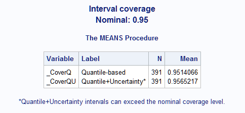
     proc genmod data=autompg;
       where cylinders in (4,6,8);
       class cylinders;
       model mpg = cylinders|weight;
       output out=MPGpreds p=p l=lclm u=uclm;
       run;

After defining the GLMPI macro in your SAS session, the macro is called as follows to compute 95% quantile-based prediction intervals for each observation (vehicle) in the data set. The contents of the input data set (MPGpreds) and the prediction interval limits are saved in the out= data set, named GLM_PI by default. Since GENMOD assumed that the response distribution is normal, dist=normal genmod is specified. The estimate of the scale parameter is provided in the Parameter Estimates table displayed by GENMOD and is found to equal 3.9749. To obtain quantile-based intervals that include uncertainty in the mean, type=all (the default) is specified. These intervals require that confidence intervals for the mean be requested in GENMOD and specified in lower= and upper=. If not provided, only intervals not including mean uncertainty are computed. In order to compute the prediction interval coverage proportion, response= must be specified in addition to options=cover.

     %glmpi(data=MPGpreds, response=mpg, dist=normal genmod, scale=3.9749, 
            pred=p, lower=lclm, upper=uclm, type=all, options=cover)  

The coverage proportion is 0.9514 for the quantile-based intervals and somewhat larger, 0.9565, for the intervals that include mean uncertainty.

These statements plot the data points and show the confidence intervals for the mean (shaded regions), quantile-based prediction intervals for future values (wide-dashed lines), and quantile-based prediction intervals including mean uncertainty (small-dashed lines).

     proc sort data=glm_pi; 
       by weight;
       run;
     proc sgpanel data=glm_pi noautolegend;
       panelby cylinders / columns=3;
       band upper=uclqu lower=lclqu x=weight / legendlabel="95% quantile PI w/ mean uncertainty" 
            name="qu" nofill lineattrs=(pattern=2 color=purple);
       band upper=uclq lower=lclq x=weight / legendlabel="95% quantile PI"
            name="q" nofill lineattrs=(pattern=4 color=black);
       band upper=uclm lower=lclm x=weight / legendlabel="95% CI for the mean" name="ci";
       reg y=p x=weight / nomarkers;
       scatter y=mpg x=weight;
       colaxis grid; rowaxis grid;
       keylegend "ci" "q" "qu";
       title "GENMOD Fit for MPG";
       title2 "With 95% Confidence and Quantile-Based Prediction Intervals";
       run;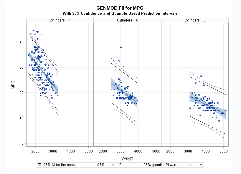

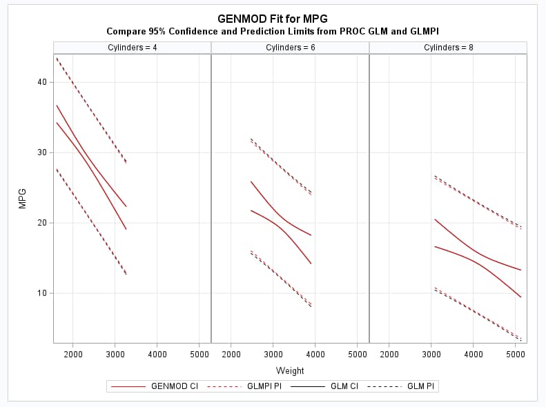
For this normal, identity-linked model, confidence and prediction intervals can also be computed by the GLM and REG procedures. The intervals produced by the GLMPI macro are essentially the same as those from PROC GLM for this model. However, since GLM uses least squares estimation rather than maximum likelihood estimation as in PROC GENMOD, their variance estimates differ slightly. Also, the intervals in GLM use a quantile from the t distribution rather than from the standard normal distribution as in GENMOD.

These statements fit the model in PROC GLM and add its 95% confidence and prediction limits to the GLM_PI data set.

     proc glm data=glm_pi plots=none;
       where cylinders in (4,6,8);
       class cylinders;
       model mpg = cylinders|weight;
       output out=glmout p=pglm lcl=lpiglm ucl=upiglm lclm=lclmglm uclm=uclmglm;
       run; quit;

These statements produce a plot that compares the confidence intervals on the mean from GENMOD and GLM as well as the prediction intervals from GLM and the GLMPI macro.

     proc sgpanel data=glmout noautolegend;
       panelby cylinders / columns=3;
       band upper=upiglm lower=lpiglm x=weight / legendlabel="GLM PI"
            name="glmpi" nofill lineattrs=(pattern=2 color=black);
       band upper=uclmglm lower=lclmglm x=weight / legendlabel="GLM CI"
            name="glmci" nofill lineattrs=(pattern=1 color=black);
       band upper=uclq lower=lclq x=weight / legendlabel="GLMPI PI"
            name="macpi"  nofill lineattrs=(pattern=2 color=red);
       band upper=uclm lower=lclm x=weight / legendlabel="GENMOD CI"
            name="genci" nofill lineattrs=(pattern=1 color=red);
       colaxis grid; rowaxis label="MPG" grid;
       keylegend "genci" "macpi" "glmci" "glmpi";
       title "GENMOD Fit for MPG";
       title2 "Compare 95% Confidence and Prediction Limits from PROC GLM and GLMPI";
       run;

As shown in the graph, the intervals in each pair are essentially identical.

EXAMPLE 2: Overdispersed count data

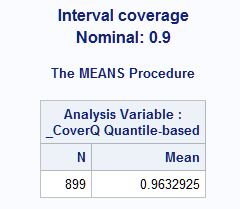
This example uses data on the number of scientific articles published by doctoral candidates appearing in examples in the COUNTREG procedure documentation. A link to the data is provided in the examples. The following statements use PROC FMM to fit a generalized Poisson model to the number of articles, ART, and save the statistics needed by the GLMPI macro. The FEM and MAR predictors are binary variables, the KID5 variable has four levels (a fifth level with few observations is omitted by the WHERE statement), and MENT is a continuous variable. The generalized Poisson model is often used to model over- or under-dispersed data as discussed in this note and illustrated in this note. The GLMPI macro is called to compute quantile-based prediction intervals. 90% confidence intervals are requested by alpha=0.1. The coverage proportion of the prediction intervals is requested by options=cover.

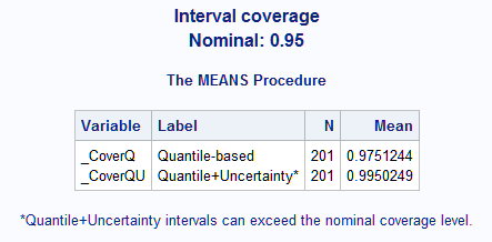
     proc fmm data=long97data;
       where kid5 ne 3;
       model art = fem mar kid5 ment / dist=genpoisson;
       id art fem mar kid5 ment;
       output out=out pred=p;
       run;
     %glmpi(data=out, response=art, dist=genpoisson fmm, scale=0.3026,
            pred=p, alpha=0.1, options=cover)

The coverage proportion, 0.96, is higher than the nominal level, 0.90 as requested by alpha=0.1. This is probably due to the large proportion of the data clustered near the zero minimum response value. The coverage would approach the nominal level with increased sample size assuming correct estimates of the distribution parameters.

These statements plot the model fit and the quantile-based prediction intervals in the various populations defined by the levels of FEM, MAR, and KID5.

     proc sort data=glm_pi; 
       by ment;
       run;
     proc sgpanel data=glm_pi noautolegend;
       panelby fem mar kid5 / columns=4;
       band upper=uclq lower=lclq x=ment;
       scatter y=art x=ment;
       loess y=p x=ment;
       title "Generalized Poisson Fit to Article Data";
       title2 "With 95% Quantile-based Prediction Limits";
       rowaxis label="Number articles";
       colaxis label="Number mentor articles";
       run;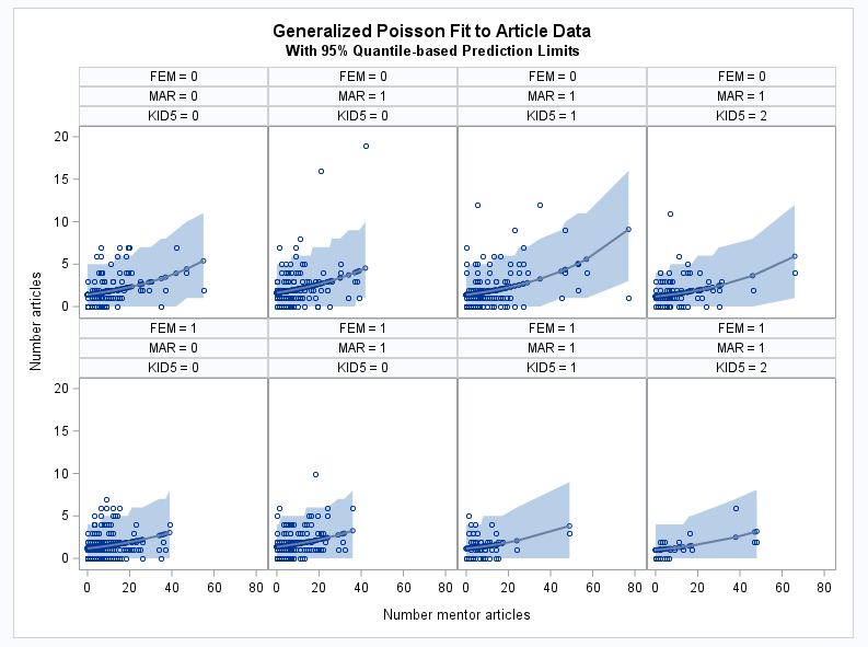

EXAMPLE 3: Gamma model

The following extends the example titled "Gamma Distribution Applied to Life Data" in the GENMOD procedure documentation. A link to the data is provided in the example. The data represent failure times of machine parts made by two manufacturers. The following statements use the GLIMMIX procedure to fit a model assuming a gamma distribution for the response variable. The GLMPI macro is called to compute 95% prediction intervals that omit and include mean uncertainty. To obtain predicted mean values and confidence limits for the mean, the ILINK suboption is used in the PRED=, LCL=, and UCL= options in the OUTPUT statement. The estimated gamma scale parameter is found in the Parameter Estimates table displayed by S option in PROC GLIMMIX (not shown).

     proc glimmix data=lifdat;
       class mfg;
       model lifetime = mfg / dist=gamma link=log s;
       output out=out pred(ilink)=p lcl(ilink)=lower ucl(ilink)=upper;
       run;
     %glmpi(data=out,response=lifetime,dist=gamma glimmix,scale=1.2085,
            pred=p,lower=lower,upper=upper,options=cover)

The coverage proportion, 0.975, is higher than the default nominal level, 0.95. This is probably due to the clustering near the zero minimum response value. The coverage would approach the nominal level with increased sample size assuming correct estimates of the distribution parameters.

These statements plot the data and show the confidence and prediction intervals for each manufacturer.

     proc sgplot data=glm_pi;
       highlow y=mfg low=lclq high=uclq / type=bar name="PI" 
               legendlabel="95% PI" fillattrs=(color=lightgrey);
       highlow y=mfg low=lower high=upper / type=bar name="CI" 
               legendlabel="95% CI" fillattrs=(color=darkgrey);
       highlow y=mfg low=p high=p / type=bar name="Mean" 
               legendlabel="Mean" fillattrs=(color=black);
       scatter y=mfg x=lifetime;
       title "Gamma Fit to Lifetime Data";
       title2 "With 95% Confidence and Quantile Prediction Limits";
       xaxis label="Lifetime";
       keylegend "Mean" "CI" "PI";
       run;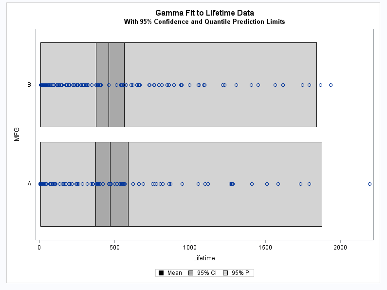

Right-click on the link below and select Save to save the GLMPI macro definition to a file. It is recommended that you name the file glmpi.sas.

Download and save glmpi.sas

The GLMPI macro computes 100(1-α)% prediction intervals using quantiles of the specified response distribution. A wide range of distributions is supported. Intervals that include uncertainty in the mean estimate are also available.

Type:	Sample
Topic:	Analytics ==> Categorical Data Analysis Analytics ==> Regression SAS Reference ==> Macro

Date Modified:	2022-11-23 16:22:21
Date Created:	2022-11-16 13:29:23

Operating System and Release Information

Product Family	Product	Host	SAS Release
			Starting	Ending
SAS System	N/A	Aster Data nCluster on Linux x64
		DB2 Universal Database on AIX
		DB2 Universal Database on Linux x64
		Netezza TwinFin 32-bit SMP Hosts
		Netezza TwinFin 32bit blade
		Netezza TwinFin 64-bit S-Blades
		Netezza TwinFin 64-bit SMP Hosts
		Teradata on Linux
		Cloud Foundry
		64-bit Enabled AIX
		64-bit Enabled HP-UX
		64-bit Enabled Solaris
		ABI+ for Intel Architecture
		AIX
		HP-UX
		HP-UX IPF
		IRIX
		Linux
		Linux for AArch64
		Linux for x64
		Linux on Itanium
		OpenVMS Alpha
		OpenVMS on HP Integrity
		Solaris
		Solaris for x64
		Tru64 UNIX
		z/OS
		z/OS 64-bit
		IBM AS/400
		OpenVMS VAX
		N/A
		Android Operating System
		Apple Mobile Operating System
		Chrome Web Browser
		Macintosh
		Macintosh on x64
		Microsoft Windows 10
		Microsoft Windows 7
		Microsoft Windows 8 Enterprise 32-bit
		Microsoft Windows 8 Enterprise x64
		Microsoft Windows 8 Pro 32-bit
		Microsoft Windows 8 Pro x64
		Microsoft Windows 8 x64
		Microsoft Windows Server 2008 R2
		Microsoft Windows Server 2012 R2 Datacenter
		Microsoft Windows Server 2012 R2 Std
		Microsoft® Windows® for 64-Bit Itanium-based Systems
		Microsoft Windows Server 2003 Datacenter 64-bit Edition
		Microsoft Windows Server 2003 Enterprise 64-bit Edition
		Microsoft Windows XP 64-bit Edition
		Microsoft® Windows® for x64
		OS/2
		SAS Cloud
		Microsoft Windows 8.1 Enterprise 32-bit
		Microsoft Windows 8.1 Enterprise x64
		Microsoft Windows 8.1 Pro 32-bit
		Microsoft Windows 8.1 Pro x64
		Microsoft Windows 11
		Microsoft Windows 95/98
		Microsoft Windows 2000 Advanced Server
		Microsoft Windows 2000 Datacenter Server
		Microsoft Windows 2000 Server
		Microsoft Windows 2000 Professional
		Microsoft Windows NT Workstation
Microsoft Windows Server 2003 Datacenter Edition
Microsoft Windows Server 2003 Enterprise Edition
Microsoft Windows Server 2003 Standard Edition
Microsoft Windows Server 2003 for x64
Microsoft Windows Server 2008
Microsoft Windows Server 2008 for x64
Microsoft Windows Server 2012 Datacenter
Microsoft Windows Server 2012 Std
Microsoft Windows Server 2016
Microsoft Windows Server 2019
Microsoft Windows Server 2022
Microsoft Windows XP Professional
Windows 7 Enterprise 32 bit
Windows 7 Enterprise x64
Windows 7 Home Premium 32 bit
Windows 7 Home Premium x64
Windows 7 Professional 32 bit
Windows 7 Professional x64
Windows 7 Ultimate 32 bit
Windows 7 Ultimate x64
Windows Millennium Edition (Me)
Windows Vista
Windows Vista for x64