Usage Note 68202: Models for continuous nonnegative response data that contain many zeros
 |  |  |
When you are modeling a positive continuous response variable that can also contain some, and possibly many, zero values, the question of an appropriate distribution arises. This type of variable is common in cost data such as total claim amounts from insurance policyholders or patient health care costs. Other examples include amounts of rainfall over multiple periods or locations, amounts of consumption of alcohol or other substances by individuals, and so on.
In the case of a discrete count response, the Poisson and negative binomial distributions are often used, and if more zeros occur than are expected under those distributions, zero-inflated Poisson and negative binomial distributions are available. Excess zeros can be a cause of overdispersion in models for count data as discussed in this note. These models can be fit in the HPGENSELECT, GENMOD, and other procedures. (See "Zero-inflated models" in this note.) The generalized Poisson distribution is another distribution for discrete count data that can be used for under- or overdispersed data. This distribution is described in more detail in the example titled Generalized Poisson Mixed Model for Overdispersed Count Data in the GLIMMIX procedure documentation and is also illustrated in this note. Models using this distribution can be fit most easily in the FMM procedure, but can also be fit with some programming in the GLIMMIX and NLMIXED procedures. When the above distributions are used for a continuous response, the modeling procedure might note that noninteger values of the response are detected but fitting of the model continues. Since these distributions are really discrete distributions, they are not technically appropriate for a continuous response but might have practical value.
For a positive continuous variable, the gamma or inverse Gaussian distributions initially might seem like choices, but zero is not a valid value under either of these distributions. Gamma and inverse Gaussian models can be fit in PROC GENMOD, and other procedures, but observations with zero response value are ignored and do not contribute to the model fit.
A distribution that supports a positive continuous response and allows for a point mass of observed zeros is the Tweedie distribution. A detailed description of the Tweedie model can be found in the "Details: Tweedie Distribution for Generalized Linear Models" section of the PROC GENMOD documentation. The Tweedie model can be fit in the GENMOD, HPGENSELECT, and GAMPL procedures and a few others. Another possibility is a model based on a modification of the gamma likelihood that allows zero values and which is discussed below.
Finally, an approach used for loss data, such as from an insurance company, is to estimate the distribution of loss using a combination of frequency of loss and severity of loss data. The resulting compound distribution model (CDM) can then be simulated in order to estimate the probability of loss, percentiles of loss, and so on. This approach is available in the HPCDM procedure. However, if interest lies in predicting the response value, such as total loss, for individual cases or groups of cases, one of the modeling approaches mentioned above can be simpler.
Several of the models discussed above are illustrated in the following example.
Example: Total losses from insurance claims
See the Getting Started example for PROC HPCDM in the SAS/ETS® Sample Library, which provides the SAS® statements that generate the data for this example and performs the CDM analysis discussed later. The data in the LOSSES data set represent loss amounts from the policyholders of an automobile insurance company over a period of one year. Predictors of the loss amount include age, gender, education level, and income of the policyholder as well as type and safety rating of the car and annual miles driven. The observations in the data set are the individual claims made. Some policyholders might have no claims within the year, or possibly one or more claims. Of interest is the total loss from each policyholder, so the following statements sum the loss amounts from multiple claims within a policyholder to produce a total loss variable to be modeled and predicted. The summarized data set, TOTLOSS, contains one observation for each policyholder. The TOTLOSS variable contains the total amount lost by the insurance company to that policyholder over the year.
     proc summary data=losses nway;
        class policyholderid;
        var lossamount carType carSafety income;
        output out=totloss sum(lossamount)=totloss
               mean(age gender carType annualMiles education  carSafety income)=;
        run;
     data totloss; set totloss;
        if totloss=. then totloss=0;
        run;
Tweedie model
The following statements fit a Tweedie model to the total loss as a function of the above predictors. The default link function used is the log link. The STORE statement saves the fitted model for use later. The raw loss residuals (actual - predicted) are computed by the OUTPUT statement and saved in the OUT= data set.
     proc genmod data=totloss;
        model totloss = age gender carType annualMiles education carSafety income / dist=tweedie;
        output out=outtw pred=predmean resraw=res;
        store twmod;
        run;
These statements compute the generalized R2 described in this note. It is used as a statistic to compare the fit of this model to other models considered below. For this purpose, the simpler, average-based version of this statistic is used so that a common baseline is used for all models.
     proc sql;
       select 1-(uss(res)/css(totloss)) as Rsquare from outtw;
       quit;
For the Tweedie model, R2 = 0.581.
The example in the HPCDM documentation then uses simulation from the estimated loss distribution to estimate the total loss for a policyholder with particular values on the predictor variables. The predictor values are in the SinglePolicy data set. The following statements use the Tweedie model saved by the STORE statement to obtain the predicted loss incurred by the policyholder. The ILINK option applies the inverse of the log link so that the predicted value is on the scale of the TOTLOSS response.
     proc plm restore=twmod noprint;
        score data=SinglePolicy out=singlepred pred stderr lclm uclm / ilink;
        run;
     proc print noobs;
        run;
The loss for this policyholder predicted by PROC HPCDM is 212 or 214, depending on the distribution used to model the loss severity. The predicted loss for the policyholder from the Tweedie model is 199 with 95% confidence interval (171, 232). Note that the predicted loss is the estimated mean of the Tweedie distribution for the population defined by the predictor values from this policyholder.
The estimated parameters of the Tweedie distribution can then be used to estimate loss percentiles. Of typical interest are the sizes of large losses that could occur, such as at the 75th and 97.5th percentiles. The following statements use the QUANTILE function in the DATA step to compute these percentiles of the Tweedie distribution for the population defined by the setting of the predictors for this policyholder. The required parameters are the mean, power, and dispersion parameters of the distribution. The mean is provided by the PLM procedure above. The power and dispersion parameters are displayed by PROC GENMOD in the table of parameter estimates of the fitted model. The estimated power parameter is 1.5019 and the estimated dispersion parameter is 47.8768.
     data pctl;
       do Percentile = .75, .975;
          Estimate = quantile('Tweedie', Percentile, 1.5019, 199, 47.8768);
          output;
       end;
       run;
     proc print;
       id Percentile;
       var Estimate;
       title "Loss percentiles for Policyholder";
       run;
The computed 75th and 97.5th loss percentiles, 261 and 1278, are similar to those computed by PROC HPCDM using two different distributions for loss severity.
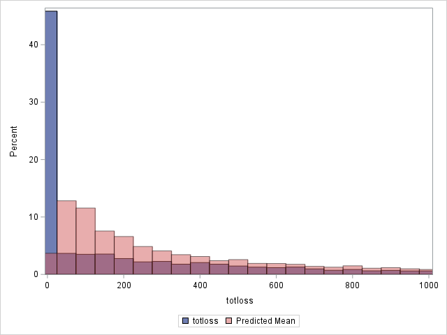
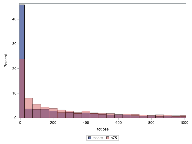
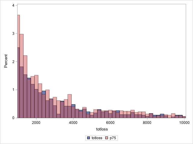
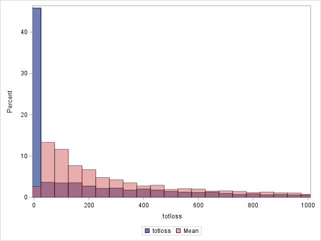
The following statements compare the overall actual and predicted distributions of loss values for these data. Separate histograms are created for two ranges of loss.
proc sgplot data=outtw;
histogram totloss / binwidth=50;
histogram predmean / binwidth=50 transparency=.5;
xaxis min=0 max=1000;
label predmean="Predicted Mean";
run;
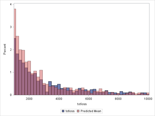
proc sgplot data=outtw;
histogram totloss / binwidth=200;
histogram predmean / binwidth=200 transparency=.5;
xaxis min=1000 max=10000;
yaxis min=0 max=4;
label predmean="Predicted Mean";
run;
Note that the proportion of predicted means at and very near zero (the first bar) is underestimated while loss is overestimated at higher loss values.
|
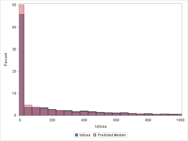
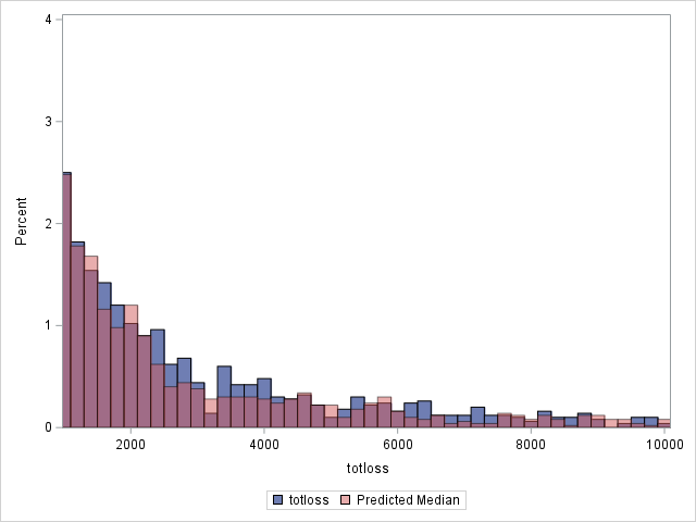
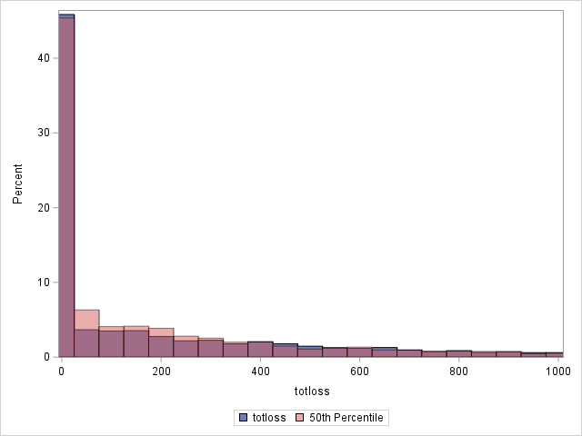
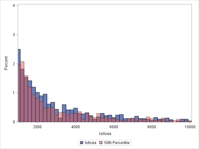
Since loss has a highly skewed distribution, it might be of interest to use something other than the means as predicted values. If the median is computed for each observation, the histograms change as shown below. Note that the predicted distribution of the medians more closely matches the observed distribution of losses. Using residuals based on the median, the generalized R2 decreases slightly to 0.562.
|
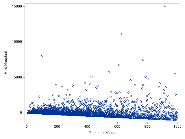
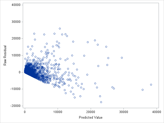
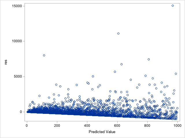
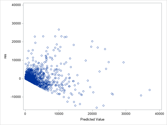
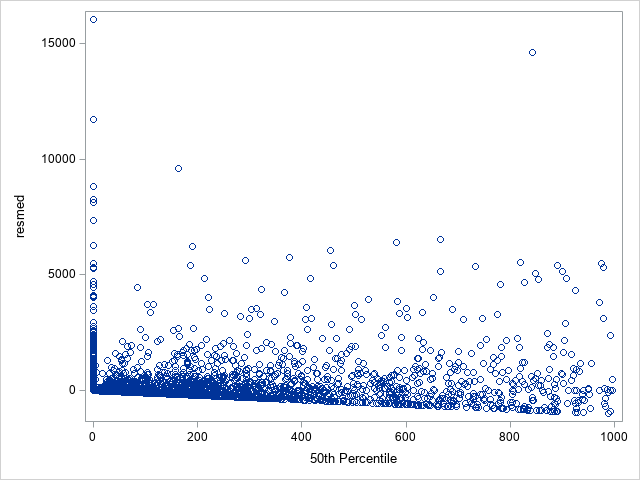
The following statements show the loss residuals based on the predicted mean under the Tweedie model. The first plot focuses on small predicted loss values (0 to 1000). The second plot shows all predicted and residual values below 40,000, excluding two values to improve resolution for the rest of the plot.
     proc sgplot data=outtw;
        where p<=1000;
        scatter y=res x=predmean;
        run;
     proc sgplot data=outtw;
        scatter y=res x=predmean;
        yaxis max=40000;
        xaxis max=40000;
        run;
Note that the Tweedie model never produces a predicted mean exactly equal to zero. So, for observations with zero observed loss, the residual is always negative. This result is seen as the apparent linear boundary of negative residuals. Residual plots using the median look very similar.
|
Zero-inflated negative binomial model
Although the negative binomial distribution and the zero-inflated version of that distribution are discrete distributions for integer-valued responses like counts, the following statements can be used to fit the model to these continuous data. A detailed description of the zero-inflated negative binomial model can be found in "Zero-Inflated Models" in the "Details" section of the PROC GENMOD documentation. The default link function is again the log link for the mean of the negative binomial component of the model. The default logit link is used for the extra zeros component of the model. Two of the predictors are found to not significantly contribute to the model for extra zeros and are therefore omitted from the ZEROMODEL statement. The STORE statement saves the fitted model.
     proc genmod data=totloss;
        model totloss = age gender carType annualMiles education carSafety income / dist=zinb;
        zeromodel age gender carType annualMiles education;
        store zinb;
        output out=zinbout resraw=res;
        run;
Using the saved model in PROC PLM as done above for the Tweedie model, the predicted loss for the single policyholder is 222 with 95% confidence interval (188, 263).
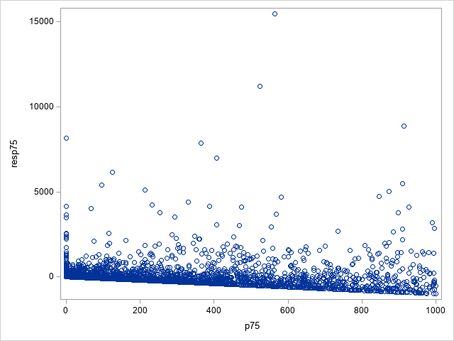
The generalized R2 computed using the mean, median, and 75th percentile are 0.495, 0.381, and 0.548 respectively. Following are histograms and residual plots using the 75th percentile. These are similar to, but perhaps not quite as good as, the Tweedie model using the median as the predicted value.
|
Modified gamma model
As noted above, the gamma model is often used for a positive continuous response. However, zero values are not in the support of that distribution and are omitted by the modeling procedure. An option is to modify the gamma deviance to allow zeros. By removing the appearance of log(y) from the deviance, the following statements maximize the negative of the resulting modified deviance. Exponentiation of the linear predictor indicates that the log link is used as is done for the other models considered here.
Since PROC PLM cannot be used to score new observations from a model fit with PROC NLMIXED, the first DATA step below adds the single policyholder observation to the top of the TOTLOSS data set. Since its response value is missing in the resulting data set, it does not influence the fit of the model. However, the PREDICT statement computes predicted values for it and all of the observations and saves them in the data set NLOUT in a variable named PRED by default. Residuals are computed in the second DATA step.
     data SP_Totloss;
        set singlepolicy totloss;
        run;
     proc nlmixed data=SP_Totloss;
        mean=exp(b0+bage*age + bgender*gender + bctype*cartype + bam*annualmiles +
                 bed*education + bcsaf*carsafety + bin*income);
        dev=-log(mean)-totloss/mean;
        model totloss ~ general(dev);
        predict mean out=nlout;
        run;
     data nlout;
       set nlout;
       res=totloss-pred;
       run;
These statements display the predicted value and confidence interval for the single policyholder. The predicted value is 190 with 95% confidence interval (169, 210).
     proc print data=nlout(obs=1) noobs;
        var pred stderrpred lower upper;
        run;
Because the deviance was modified, this model is no longer based strictly on an underlying probability distribution. As a result, quantiles cannot be computed. Using the residuals, the generalized R2 is computed as before, yielding a value of 0.576. Following are histograms and residual plots. The generalized R2 value and these plots are quite similar to the Tweedie model using the mean. However, using the Tweedie median as the predicted value still shows better agreement with the observed data at lower values.
|


Generalized Poisson model
Ignoring the fact that the generalized Poisson is a distribution for a discrete, integer-valued response, the following statements fit the model using that distribution. The conjugate-gradient optimization fitting method (TECH=CONGRA) is used since it provides better convergence for these data and model. As with the modified gamma model above, PROC PLM cannot be used to score new observations, so the single policyholder observation is added to the original data before fitting the model. Predicted means are then computed for all observations and saved in the data set OUTFMM. Residuals for the original data are also computed and saved.
     proc fmm data=SP_Totloss tech=congra;
        model totloss = age gender carType annualMiles education carSafety income / dist=genpoisson;
        output out=outfmm pred=p resid=res;
        run;
The following statements display the observation for the single policyholder. Its predicted value is 196. No standard error or confidence interval is available.
     proc print data=outfmm(obs=1) noobs;
        run;
The DATA step that follows transforms the mean and scale parameters in the parameterization of the generalized Poisson distribution used in PROC FMM to theta (θ) and eta (η) in the parameterization used in the QUANTILE function. It then computes the predicted medians, 85th percentiles, and residuals based on those quantiles and adds them to the data set.
     data outfmm; set outfmm;
        scale=5.4796; theta=p*exp(-scale); eta=1-exp(-scale);
        med=quantile("genpoisson",0.5,theta,eta);
        p85=quantile("genpoisson",0.85,theta,eta);
        resmed=totloss-med; resp85=totloss-p85;
        drop scale;
        run;
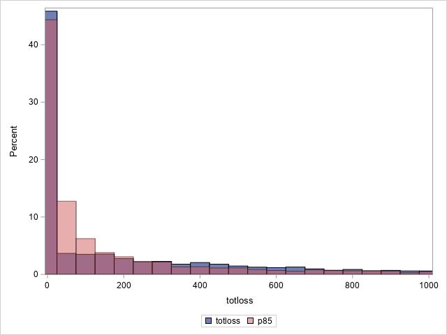
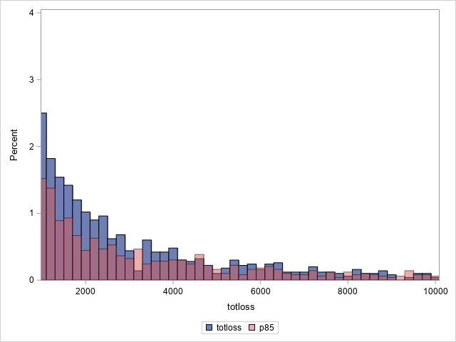
Using the computed residuals, the generalized R2 values are 0.364, 0.166, and 0.557 when the mean, median, and 85th percentile, respectively, are used. That suggests that the fit of the generalized Poisson model using the 85th percentile as the predicted value is comparable to the fit of the Tweedie and CDM (see below) for these data. The histograms comparing the distribution using the 85th percentile to the distribution of actual values shows fairly good agreement, though perhaps not as good as from the Tweedie model using the median.
|
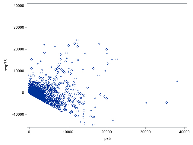
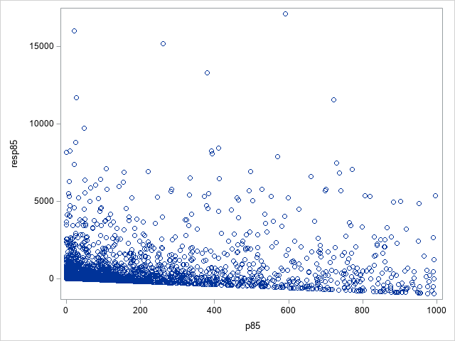
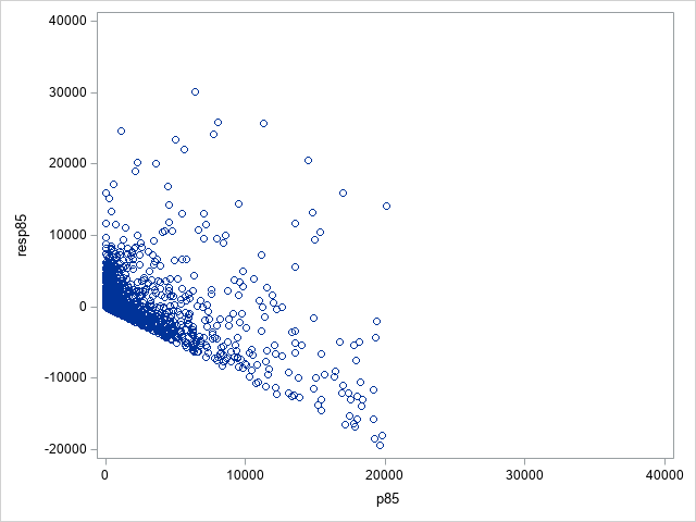
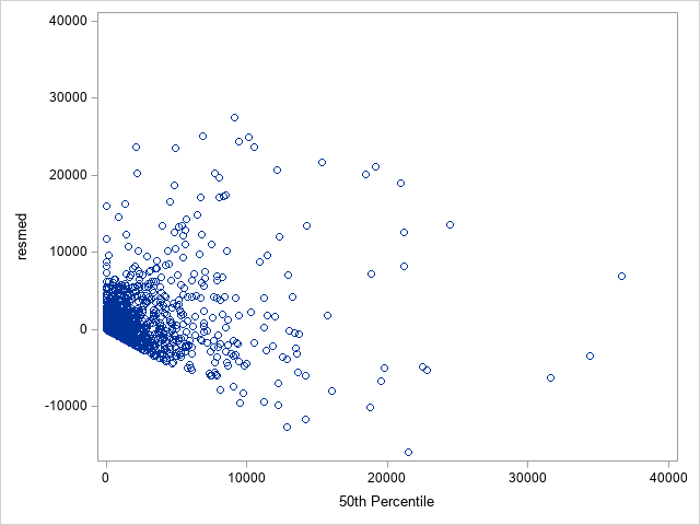
Following are plots of the residuals based on the 85th percentile, both below 1000 and overall. The residuals at lower values of the 85th percentile are somewhat larger than seen from the Tweedie and compound distribution models.
|
Comparison to the CDM from PROC HPCDM
The discussion of this example in the "Getting Started: Scenario Analysis" section of the PROC HPCDM documentation shows how the CDM can be used to simulate the loss distribution for a policyholder with a given set of predictor values. Estimates of the mean, median, or other quantiles of the loss distribution are then available. If that process is repeated for all policyholders in the data set, the mean and median can be obtained for each policyholder along with residuals based on those statistics. If a data set is created containing those values, then the generalized R-square can be computed as above. The R2 computed for the CDM is 0.583 using the mean or 0.562 using the median. Those values are similar to the value produced by the Tweedie model.
As for the earlier models, histograms can be created of the overall observed loss distribution for these policyholders and compared to the distribution of loss under the CDM using both the mean and the median. As with the Tweedie model, the median seems to serve better as a predicted value.
|

Residual plots for the CDM based on the mean are very similar to plots above for the Tweedie model. Following are plots of residuals based on the median for the CDM. Somewhat larger residuals are seen at low values since medians tend to be smaller than means in this skewed distribution.
|
Operating System and Release Information
| Product Family | Product | System | SAS Release | |
| Reported | Fixed* | |||
| SAS System | N/A | 64-bit Enabled HP-UX | ||
| DB2 Universal Database on AIX | ||||
| DB2 Universal Database on Linux x64 | ||||
| Aster Data nCluster on Linux x64 | ||||
| 64-bit Enabled AIX | ||||
| Netezza TwinFin 32bit blade | ||||
| Netezza TwinFin 32-bit SMP Hosts | ||||
| Teradata on Linux | ||||
| Cloud Foundry | ||||
| Netezza TwinFin 64-bit SMP Hosts | ||||
| 64-bit Enabled Solaris | ||||
| Netezza TwinFin 64-bit S-Blades | ||||
| ABI+ for Intel Architecture | ||||
| AIX | ||||
| HP-UX | ||||
| HP-UX IPF | ||||
| IRIX | ||||
| Linux | ||||
| Linux for AArch64 | ||||
| Linux for x64 | ||||
| Linux on Itanium | ||||
| OpenVMS Alpha | ||||
| OpenVMS on HP Integrity | ||||
| Solaris | ||||
| Solaris for x64 | ||||
| Tru64 UNIX | ||||
| z/OS | ||||
| z/OS 64-bit | ||||
| IBM AS/400 | ||||
| OpenVMS VAX | ||||
| N/A | ||||
| Android Operating System | ||||
| Apple Mobile Operating System | ||||
| Chrome Web Browser | ||||
| Macintosh | ||||
| Macintosh on x64 | ||||
| Microsoft Windows 10 | ||||
| Microsoft Windows 7 | ||||
| Microsoft Windows 8 Enterprise 32-bit | ||||
| Microsoft Windows 8 Enterprise x64 | ||||
| Microsoft Windows 8 Pro 32-bit | ||||
| Microsoft Windows 8 Pro x64 | ||||
| Microsoft Windows 8 x64 | ||||
| Microsoft Windows Server 2008 R2 | ||||
| Microsoft Windows Server 2012 R2 Datacenter | ||||
| Microsoft Windows Server 2012 R2 Std | ||||
| Microsoft® Windows® for 64-Bit Itanium-based Systems | ||||
| Microsoft Windows Server 2003 Datacenter 64-bit Edition | ||||
| Microsoft Windows Server 2003 Enterprise 64-bit Edition | ||||
| Microsoft Windows XP 64-bit Edition | ||||
| Microsoft® Windows® for x64 | ||||
| OS/2 | ||||
| SAS Cloud | ||||
| Microsoft Windows 8.1 Enterprise 32-bit | ||||
| Microsoft Windows 8.1 Enterprise x64 | ||||
| Microsoft Windows 8.1 Pro 32-bit | ||||
| Microsoft Windows 8.1 Pro x64 | ||||
| Microsoft Windows 95/98 | ||||
| Microsoft Windows 2000 Advanced Server | ||||
| Microsoft Windows 2000 Datacenter Server | ||||
| Microsoft Windows 2000 Server | ||||
| Microsoft Windows 2000 Professional | ||||
| Microsoft Windows NT Workstation | ||||
| Microsoft Windows Server 2003 Datacenter Edition | ||||
| Microsoft Windows Server 2003 Enterprise Edition | ||||
| Microsoft Windows Server 2003 Standard Edition | ||||
| Microsoft Windows Server 2003 for x64 | ||||
| Microsoft Windows Server 2008 | ||||
| Microsoft Windows Server 2008 for x64 | ||||
| Microsoft Windows Server 2012 Datacenter | ||||
| Microsoft Windows Server 2012 Std | ||||
| Microsoft Windows Server 2016 | ||||
| Microsoft Windows Server 2019 | ||||
| Microsoft Windows XP Professional | ||||
| Windows 7 Enterprise 32 bit | ||||
| Windows 7 Enterprise x64 | ||||
| Windows 7 Home Premium 32 bit | ||||
| Windows 7 Home Premium x64 | ||||
| Windows 7 Professional 32 bit | ||||
| Windows 7 Professional x64 | ||||
| Windows 7 Ultimate 32 bit | ||||
| Windows 7 Ultimate x64 | ||||
| Windows Millennium Edition (Me) | ||||
| Windows Vista | ||||
| Windows Vista for x64 | ||||
| Type: | Usage Note |
| Priority: | |
| Topic: | Analytics ==> Regression SAS Reference ==> Procedures ==> FMM SAS Reference ==> Procedures ==> GENMOD SAS Reference ==> Procedures ==> HPCDM SAS Reference ==> Procedures ==> NLMIXED |
| Date Modified: | 2021-08-31 13:59:00 |
| Date Created: | 2021-08-03 15:48:35 |