Precision-recall curve for imbalanced, rare event data

Contents:

Purpose / History / Requirements / Usage / Details / Missing Values / See Also / References

 

Note: Beginning in SAS^® Viya^® platform 2022.09, PROC LOGISTIC can plot the precision-recall curve, compute the area beneath it, and find optimal points using two criteria.

PURPOSE:

The PRcurve macro plots the precision-recall curve, computes the area beneath it, and can find optimal points on the curve that correspond to maximized values of the F score and Matthews correlation coefficient criteria.

HISTORY:

The version of the PRcurve macro that you are using is displayed when you specify version (or any string) as the first argument. Here is an example:

    %prcurve(version, <other options>)

The PRcurve macro always attempts to check for a later version of itself. If it is unable to do this (such as if there is no active internet connection available), the macro issues the following message:

   NOTE: Unable to check for newer version

The computations that are performed by the macro are not affected by the appearance of this message.

Version	Update Notes
1.1	Print Note if SAS/ETS® is not available for computing/displaying area under PR curve.
1.0	Initial coding

REQUIREMENTS:

Base SAS^®. Data required by the macro must be created by the LOGISTIC procedure in SAS/STAT^®. SAS/ETS^® software is required when options=area is specified.

USAGE:

Follow the instructions on the Downloads tab of this sample to save the PRcurve macro definition. Replace the text within quotation marks in the following statement with the location of the PRcurve macro definition file on your system. In your SAS program or in the SAS editor window, specify this statement to define the PRcurve macro and make it available for use:

   %inc "<location of your file containing the PRcurve macro>";

Following this statement, you can call the PRcurve macro. See the Results tab for examples.

The following parameters are available in the PRcurve macro:

data=data-set-name

Specifies the name of a data set created by either the OUTROC= option or the CTABLE option in PROC LOGISTIC. If the available data consists only of actual responses and predicted event probabilities from a model or classifier, then use PROC LOGISTIC to create the OUTROC= data set by using the PRED= option in the ROC statement to read the predicted event probabilities and the NOFIT and OUTROC= options in the MODEL statement. If the data= parameter is omitted, the data set that was last created is used. Running the macro does not change the last-created data set, which means that successive runs of the macro omitting data= can operate on the same input data set.

inpred=data-set-name

Specifies the name of a data set created by the OUT= and PRED= options in the OUTPUT statement of PROC LOGISTIC. It is ignored if options=optimal and pred= are not also specified.

pred=variable-name

Specifies the name of the variable created by the PRED= option in the data set created by the OUT= option in the OUTPUT statement of PROC LOGISTIC. It is ignored if options=optimal and inpred= are not also specified.

optvars=variable-list

Specifies the names of one or more variables in the data set created by the OUT= option in the OUTPUT statement of PROC LOGISTIC that will be used to identify optimal points on the PR curve. Separate multiple variable names with spaces. Variable lists, such as x1-x9, are not supported. It is ignored if options=optimal, inpred=, and pred= are not also specified.

npoints=integer

Specifies a positive integer value representing the number of interpolated points between 0 and 1 that the macro will generate along the PR curve. The default value is npoints=100.

beta=value

Specifies a positive value representing the parameter of the F score optimality criterion. Typical values are 0.5, 1, or 2 that control the relative importance of precision and recall in the F score. It is ignored if options=optimal is not also specified. The default value is beta=1.

sensdelta=value

Specifies a small positive value that represents the minimum difference in sensitivity values between an interpolated point and a point from the data= data set. The default value is sensdelta=1e-10.

sensinc=value

Specifies a small positive value that slightly increases successive sensitivity values in the data= data set so that the area under the curve can be computed. The default value is sensinc=1e-14.

options=list-of-options

Specifies desired options separated by spaces. The default value is options=pprob area markers br ppvzero nooptimal. Valid options are as follows:

pprob | nopprob

Requests drawing a horizontal reference line at the observed, overall event proportion and displaying its value on the plot. This line represents the PR curve of a random, "no skill" model. Specifying nopprob omits the line and value.

area | noarea

Requests computation of the area below the PR curve and display of its value on the plot. Area computation requires SAS/ETS. Specify noarea to not compute or display the area.

tl | tr | bl | br

Specifies in which corner of the plot to display the area and event proportion, if requested.

markers | nomarkers

Requests the display of markers at each of the threshold points provided in the data= data set. When there are a large number of threshold points, it might be desirable to specify nomarkers.

optimal | nooptimal

Requests computation of the F score and Matthews correlation coefficient (MCC) at each threshold point in the data= data set, and if optvars= is specified, it displays a table of the optimal values and corresponding values of the variables that are specified in optvars=. Specify nooptimal if computation of optimal points is not desired.

ppvzero | noppvzero

Requests that the PR curve include a point at (0,0) when a threshold point in the data= data set contains zero true positives and nonzero false positives. Specifying noppvzero ignores such points, which results in the PR curve being constant (flat) from recall=0 to the first precision (PPV) of the first threshold point in which the number of true positives exceeds zero. The area, if requested, is affected by this choice.

DETAILS:

The Receiver Operating Characteristic (ROC) curve and the area beneath it (AUC-ROC) are perhaps the most commonly used graphic and statistic for assessing the performance of binary-response models or classifiers. However, as described by Saito and Rehmsmeier (2015) and others, the ROC curve and AUC-ROC can be misleading when the proportions of events and nonevents become very imbalanced, such as when there are very few observed events. They note that the statistics behind the ROC curve, sensitivity and specificity, are invariant to the degree of imbalance. When interest focuses on the model predicting a high proportion of true events among the predicted events, a plot involving that statistic, known as the precision or positive predictive value (PPV), can be more informative. The fact that the precision, unlike specificity, is sensitive to the degree of imbalance allows a plot of precision to more accurately reflect the measure of interest, regardless of the degree of imbalance. This is the advantage of the precision-recall (PR) curve and its area (AUC-PR).

Saito and Rehmsmeier (2015) provide a good comparison of ROC and PR curves and show that the PR curve gives a better assessment of model performance when the proportions of events and nonevents in the data are imbalanced.

Davis and Goadrich (2006) discuss how the ROC space and the PR space are related and particularly how interpolation must be done among the observed points in PR space. They note that, while linear interpolation can be used between points in ROC space, it is not the case in PR space. The PRcurve macro applies their interpolation method when plotting the PR curve and computing the area under it.

The PRcurve macro plots precision against sensitivity and computes the area under the curve (AUC-PR). It can also find optimal points on the PR curve that have maximum values on the F score and Matthews correlation coefficient (MCC). When predicted event probabilities (from inpred= and pred=) and one or more predictor variables in the model (from optvars=) are specified, the macro displays a table of the optimal points based on the above optimality criteria and the predictor values corresponding to those points.

The F score and MCC combine the precision and recall measures. A parameter, β, can be specified for the F score to control the relative balance of the importance of precision to recall. At the default, β=1, the F score is the harmonic mean of the two and they are treated as equally important. When β > 1 (β=2 is commonly used), more importance is given to recall. When β < 1 (β=0.5 is commonly used), precision is more important. The F score ranges between 0 and 1 and equals 1 when precision and recall both equal 1. MCC is considered by some to be a better statistic. It is the geometric mean of precision and recall and is equivalent to the phi coefficient. It ranges from -1 to 1 and equals 1 when all observations are correctly classified.

BY-group processing

While the PRcurve macro does not directly support BY-group processing, this capability can be provided by the RunBY macro, which can run the PRcurve macro repeatedly for each of the BY groups in your data. See the RunBY macro documentation (SAS Note 66249) for details about its use. Also see the example titled "BY-group processing" on the Results tab.

Output data sets

Two data sets are automatically created:

_PR

Contains the points on the PR curve including both those from the data= data set and the interpolated points that are generated by the macro.

_PROpt

Produced if options=optimal, inpred=, pred=, and optvars= are all specified. Contains the optimal points on the PR curve. For each, the associated values of the optimality criteria and of the variables specified in optvars= are given. When the data= data set is a CTABLE data set, the value of the threshold in the inpred= data set that most closely matches the threshold of the optimal point from the data= data set is also given.

MISSING VALUES:

Missing values should not appear in the data= data set. Missing values are tolerated in the inpred= data set and pred= variable and do not affect the results.

SEE ALSO:

The ROC curve, the area under the ROC curve, and comparisons of ROC curves and their areas are available in PROC LOGISTIC using the ROC and ROCCONTRAST statements. See the example in the LOGISTIC documentation. Comparison of independent ROC curves, such as curves fit to independent samples, is described in SAS Note 45339. Computation of optimal values on the ROC curve, using various optimality criteria, can be done using the ROCPLOT macro (SAS Note 25018).

REFERENCES:

Davis, J., and Goadrich, M.H. 2006. "The relationship between Precision-Recall and ROC curves." Proceedings of the 23rd international Conference on Machine Learning.

Fawcett, T. 2004. ROC Graphs: Notes and Practical Considerations for Researchers. Norwell, MA: Kluwer Academic Publishers.

Saito T., and Rehmsmeier M. 2015. "The Precision-Recall Plot Is More Informative Than the ROC Plot When Evaluating Binary Classifiers on Imbalanced Datasets." PLoS ONE. 10(3): e0118432.

Williams, C.K.I. 2021. "The Effect of Class Imbalance on Precision-Recall Curves." Neural Computation 33(4): 853–857.

---

These sample files and code examples are provided by SAS Institute Inc. "as is" without warranty of any kind, either express or implied, including but not limited to the implied warranties of merchantability and fitness for a particular purpose. Recipients acknowledge and agree that SAS Institute shall not be liable for any damages whatsoever arising out of their use of this material. In addition, SAS Institute will provide no support for the materials contained herein.

---

---

These sample files and code examples are provided by SAS Institute Inc. "as is" without warranty of any kind, either express or implied, including but not limited to the implied warranties of merchantability and fitness for a particular purpose. Recipients acknowledge and agree that SAS Institute shall not be liable for any damages whatsoever arising out of their use of this material. In addition, SAS Institute will provide no support for the materials contained herein.

The following examples show how the precision-recall (PR) curve can be created using either the PRcurve macro or using options available beginning in SAS Viya 4. Additional examples of plotting the PR curve, finding the area under the curve (AUC), and optionally finding optimal points on the curve using various criteria can be found in SAS Note 71200.

EXAMPLE 1: PR curve, AUC, and optimal points for logistic model

The following uses the data from the example titled "Logistic Regression" in the GENMOD documentation. PROC LOGISTIC fits the logistic model, plots the ROC curve, and saves the ROC plot data in the data set OR. The PRcurve macro then plots the precision-recall (PR) curve and computes the area under the PR curve.

    proc logistic data=drug;
      class drug;
      model r/n = drug x / outroc=or;
      run;
    %prcurve()

Equivalently in SAS Viya 4, very similar results are obtained by adding the following options in the above PROC LOGISTIC statement. Note that several methods are available for creating both the ROC and the PR curve. The LOWER method is essentially what the PRcurve macro uses. See the description of the METHOD= option in the PROC LOGISTIC documentation for SAS Viya.

    plots(only)=(roc pr) rocoptions(method=lower)

The resulting ROC plot and area under the ROC curve (AUC = 0.84) show evidence of moderately good model fit. Note that an ROC curve lying close to the diagonal line with AUC near 0.5 indicates a poorly fitting model that essentially randomly classifies observations as positive or negative. The ROC curve of a perfectly fitting model that classifies all observations correctly is a curve from (0,0) to (0,1) to (1,1) with AUC = 1.

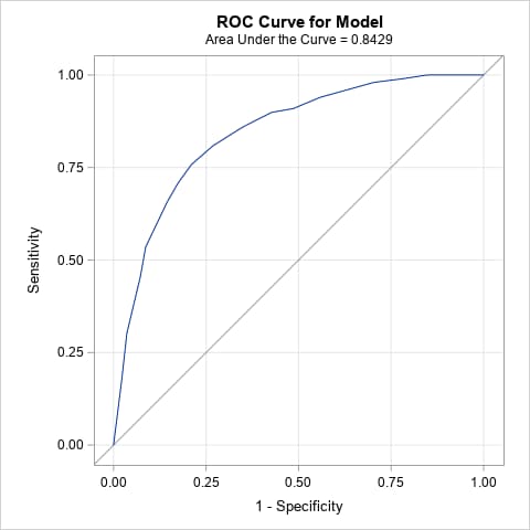
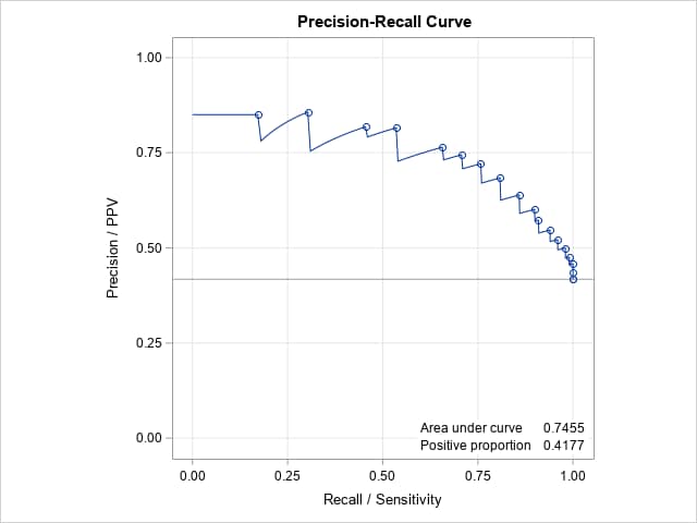
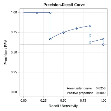
Note that the overall proportion of positives in the data is 0.42. That indicates that the positive and negative responses are reasonably balanced, making the PR curve less necessary for assessing the model. As with the ROC curve and its AUC, the PR curve and AUC = 0.75 suggest a moderately good fitting model. Note that a PR curve lying close to the horizontal, positive proportion line with AUC equal to that proportion indicates a poor, randomly classifying model. The PR curve of a model that fits and classifies perfectly is a curve from (0,1) to (1,1) to (1,0) with AUC = 1.

The following macro call computes and identifies optimal points on the PR curve and displays their corresponding thresholds on the predicted probabilities.

    %prcurve(options=optimal)

Points at the maximum F(1) score and Matthews correlation coefficient (MCC) are identified with colors on the PR curve. The achieved values on these optimality criteria and the predicted probability thresholds (cutoffs) at which they occur are given in the legend below the plot. Note that the F score using the default parameter value, β = 1, is the harmonic mean of precision and recall.

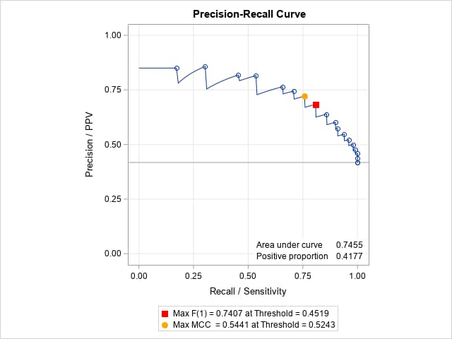
In SAS Viya, adding the option OPTIMAL=(F MCC) in ROCOPTIONS highlights the points on both the ROC and PR curves that are optimal according to the F and MCC criteria. Additional criteria are available such as the Youden and cost-based criteria. For the ROC curve only, these additional criteria are also available by using the ROCPLOT macro. If you also add the ID=OPTSTAT option in ROCOPTIONS, then the points on the ROC and PR curves are labeled with the value of the first-specified optimality criterion - in this case, the F criterion.

In order to display the predictor values corresponding to the optimal PR points, the data set containing predicted probabilities under the fitted model must be provided in inpred=. The variable containing the predicted probabilities is specified in pred=. Also, specify some or all of the predictor variables to display in optvars=. The following statements refit the model, save the necessary data sets, and repeat the previous plot:

    proc logistic data=drug;
       class drug;
       model r/n = drug x / outroc=or;
       output out=preds pred=p;
       run;
    %prcurve(data=or, inpred=preds, pred=p, options=optimal, optvars=drug x)

In addition to repeating the plot above, the following table of optimal points is displayed.

Optimal Points on the P-R Curve Optimality Statistic Optimality Value drug x Max F(1) 0.74074 B 0.78 Max MCC 0.54406 D 0.34

In SAS Viya, in order to display the achieved value of all specified criteria as well as the predictor values and cutoff probabilities at which they occur, add an ID statement listing the predictors in the model and also specify ID=ID in ROCOPTIONS. This will add all the necessary information in the OUTROC= data set for both the ROC and PR curves. You can then display the observations that contain the optimal cutoffs. For this example, the following statements display the above information for the optimal points on the F and MCC criteria.

    proc logistic data=drug plots(only)=(roc pr) 
       rocoptions(method=lower optimal=(f mcc) id=id);
       class drug;
       id drug x;
       model r/n = drug x / outroc=or;
       run;
    proc print data=or(where=(_optmcc_ or _optf1_)) noobs label; 
       id drug x;
       var _prob_ _optf1_ _f1_ _optmcc_ _mcc_;
       run;

EXAMPLE 2: PR curve for data from previous model or classifier

If a model or classifier has already been used providing a data set of actual responses and predicted event probabilities, you can use PROC LOGISTIC to create the OUTROC= data set needed by the PRcurve macro. Specify the variable containing the predicted event probabilities in the PRED= option in the ROC statement. In the MODEL statement, specify the value representing the event of interest in the EVENT= option following the response variable. Also specify the NOFIT and OUTROC= options. No predictors need to be specified.

The following simple example illustrates how this is done:

    data x; 
       input p y; 
       datalines;
    0.9 1
    0.8 1
    0.7 0
    0.6 1
    0.55 1
    0.54 1
    0.53 0
    0.52 0
    0.51 1
    0.505 0
    ;
    proc logistic data=x;
       model y(event='1')= / nofit outroc=xor;  
       roc pred=p;
       run;
    %prcurve()

Below are the ROC and PR curves for these data.

In SAS Viya, the above is done by adding the following PLOTS= option in the PROC LOGISTIC statement.

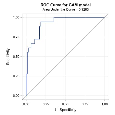
    plots(only)=(roc pr) rocoptions(method=lower)

The same can be done for a model fit by another SAS procedure that uses any modeling method appropriate for a binary response and provides a data set of the predicted event probabilities and actual responses. The ROC curve and AUC can be obtained as illustrated in SAS Note 41364. The following produces the PR curve for the Generalized Additive Model (GAM) example shown in that note. Notice that the OUTROC= option is added so that the data set can be used in the PRcurve macro. The OUT= data set from the GAM procedure is specified in inpred= to obtain optimal points on the PR curve and the corresponding predictor values.

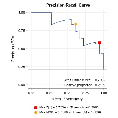
    proc gam data=Kyphosis;
       model Kyphosis(event="1") = spline(Age      ,df=3)
                                   spline(StartVert,df=3)
                                   spline(NumVert  ,df=3) / dist=binomial;
       output out=gamout predicted;
       run;
    proc logistic data=gamout;
       model Kyphosis(event="1") = / nofit outroc=gamor;
       roc "GAM model" pred=P_Kyphosis;
       run;
    %prcurve(data=gamor, inpred=gamout, pred=P_Kyphosis,
             optvars=age startvert numvert, options=optimal nomarkers)

Below is the ROC produced by PROC LOGISTIC and the PR curve from the PRcurve macro. Notice that the proportion of events (positive proportion) is 0.2169. Optimal points on the PR curve, identified by values on the three predictors in the generalized additive model, are provided following the plots.

Optimal Points on the P-R Curve Optimality Statistic Optimality Value Age StartVert NumVert Max F(1) 0.72340 82 14 5 Max MCC 0.65805 130 1 4

In SAS Viya, the following produces the ROC and PR curves and displays the optimal values and cutoff probabilities.

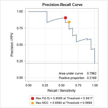
    proc logistic data=gamout plots(only)=(roc pr)
       rocoptions(optimal=(f mcc) id=id);
       id age startvert numvert;
       model Kyphosis(event="1") = / nofit outroc=gamor;
       roc "GAM model" pred=P_Kyphosis;
       run;
    proc print data=gamor(where=(_optf1_ or _optmcc_)) noobs label; 
       id age startvert numvert;
       var _prob_ _optf1_ _f1_ _optmcc_ _mcc_;
       run;

The point on the above PR curve that is optimal under the F score criterion assumes equal importance of precision (PPV) and recall (sensitivity). That is the implication of the default β = 1 parameter for the F(β) score. With β = 1, the F score computed at each threshold is the harmonic mean of precision and recall. If, however, recall is considered more important, then a larger value of β can be used. Conversely, if precision is considered more important, a smaller value of β can be used. The following finds the optimal points, under the F score criterion, for β = 0.5 and 2. For both cases, the predictor values associated with the optimal points could be identified by also specifying inpred=, pred=, optvars=, and options=optimal. Note that there is no corresponding parameter for the MCC criterion, so the optimal point under that criterion does not change.

    %prcurve(data=gamor, options=optimal nomarkers, beta=0.5)
    %prcurve(data=gamor, options=optimal nomarkers, beta=2)

Notice that the optimal point with maximum value for F(0.5) has moved to a value with considerably larger precision. However, the point optimal under F(2) did not move from the point found under the default F(1) criterion – notice the identical threshold value, 0.5699, associated with the F(1) and F(2) maxima. That threshold has a fairly large recall value under both criteria.

In SAS Viya, this is easily done by changing OPTIMAL=(F MCC) in the PROC LOGISTIC step above to OPTIMAL=(F(0.5 2) MCC). Values of the optimal cutoffs can be found in the OUTROC= data set.

EXAMPLE 3: BY-group processing

While the PRcurve macro does not support BY processing directly, the RunBY macro (SAS Note 66249) can be used to run the macro on BY groups in the data. The following uses the data in the example titled "Binomial Counts in Randomized Blocks." See the description of the RunBY macro for details about its use and links to several examples. The PROC LOGISTIC step below uses the BY statement to fit separate models to the levels of the BLOCK variable in the data and saves the ROC data. The OUTROC= data set similarly contains the BLOCK variable identifying the ROC data for each block.

    proc logistic data=HessianFly;
       by block;
       model y/n = entry / outroc=blockor;
    run;

The RunBY macro is then used to run the PRcurve macro for each block in turn. This action is done by specifying the code to be run on each BY group in a macro that you create that is named CODE. The statements below create the CODE macro containing a DATA step that includes a subsetting WHERE statement that specifies the special macro variables, _BYx and _LVLx, which are used by the RunBY macro to process each BY group. The PRcurve macro is then called to run on the subset data. The BYlabel macro variable is also used to label the displayed results from each BY group. Since the PRcurve macro writes its own titles, a FOOTNOTE statement is used instead of a TITLE statement to provide the label.

    %macro code();
       data byor; set blockor; where &_BY1=&_LVL1; run;
       footnote "Above plot for &BYlabel";
       %prcurve(data=byor)
    %mend;
    %RunBY(data=blockor, by=block)

Right-click the link below and select Save to save the PRcurve macro definition to a file. It is recommended that you name the file prcurve.sas.

Download and save prcurve.sas

The commonly used ROC curve for assessing model performance can be misleading with rare event data. The precision-recall (PR) curve is more informative in such cases. The PRcurve macro plots the PR curve, computes the area under it, and finds points corresponding to the F score and MCC criteria.

Type:	Sample
Topic:	Analytics ==> Categorical Data Analysis Analytics ==> Regression Analytics ==> Statistical Graphics

Date Modified:	2025-06-24 15:59:26
Date Created:	2021-06-23 14:51:48

Operating System and Release Information

Product Family	Product	Host	SAS Release
			Starting	Ending
SAS System	N/A	Aster Data nCluster on Linux x64
		DB2 Universal Database on AIX
		DB2 Universal Database on Linux x64
		Netezza TwinFin 32-bit SMP Hosts
		Netezza TwinFin 32bit blade
		Netezza TwinFin 64-bit S-Blades
		Netezza TwinFin 64-bit SMP Hosts
		Teradata on Linux
		Cloud Foundry
		64-bit Enabled AIX
		64-bit Enabled HP-UX
		64-bit Enabled Solaris
		ABI+ for Intel Architecture
		AIX
		HP-UX
		HP-UX IPF
		IRIX
		Linux
		Linux for AArch64
		Linux for x64
		Linux on Itanium
		OpenVMS Alpha
		OpenVMS on HP Integrity
		Solaris
		Solaris for x64
		Tru64 UNIX
		z/OS
		z/OS 64-bit
		IBM AS/400
		OpenVMS VAX
		N/A
		Android Operating System
		Apple Mobile Operating System
		Chrome Web Browser
		Macintosh
		Macintosh on x64
		Microsoft Windows 10
		Microsoft Windows 7
		Microsoft Windows 8 Enterprise 32-bit
		Microsoft Windows 8 Enterprise x64
		Microsoft Windows 8 Pro 32-bit
		Microsoft Windows 8 Pro x64
		Microsoft Windows 8 x64
		Microsoft Windows Server 2008 R2
		Microsoft Windows Server 2012 R2 Datacenter
		Microsoft Windows Server 2012 R2 Std
		Microsoft® Windows® for 64-Bit Itanium-based Systems
		Microsoft Windows Server 2003 Datacenter 64-bit Edition
		Microsoft Windows Server 2003 Enterprise 64-bit Edition
		Microsoft Windows XP 64-bit Edition
		Microsoft® Windows® for x64
		OS/2
		SAS Cloud
		Microsoft Windows 8.1 Enterprise 32-bit
		Microsoft Windows 8.1 Enterprise x64
		Microsoft Windows 8.1 Pro 32-bit
		Microsoft Windows 8.1 Pro x64
		Microsoft Windows 95/98
		Microsoft Windows 2000 Advanced Server
		Microsoft Windows 2000 Datacenter Server
		Microsoft Windows 2000 Server
		Microsoft Windows 2000 Professional
		Microsoft Windows NT Workstation
		Microsoft Windows Server 2003 Datacenter Edition
Microsoft Windows Server 2003 Enterprise Edition
Microsoft Windows Server 2003 Standard Edition
Microsoft Windows Server 2003 for x64
Microsoft Windows Server 2008
Microsoft Windows Server 2008 for x64
Microsoft Windows Server 2012 Datacenter
Microsoft Windows Server 2012 Std
Microsoft Windows Server 2016
Microsoft Windows Server 2019
Microsoft Windows XP Professional
Windows 7 Enterprise 32 bit
Windows 7 Enterprise x64
Windows 7 Home Premium 32 bit
Windows 7 Home Premium x64
Windows 7 Professional 32 bit
Windows 7 Professional x64
Windows 7 Ultimate 32 bit
Windows 7 Ultimate x64
Windows Millennium Edition (Me)
Windows Vista
Windows Vista for x64