Usage Note 67024: Assess the effect of a continuous variable using a CONTRAST or ESTIMATE statement or the Margins macro
 |  |  |
When a model contains interactions, it is often of interest to assess the effect of one of the interacting variables. When the variable of interest is categorical, and therefore is specified in the CLASS statement, its effect is the change in the response mean among its levels. This is most easily done using the LSMEANS, SLICE, or LSMESTIMATE statement. The ESTIMATE and CONTRAST statements can also be used but require you to properly determine the coefficients on the model parameters. The advantage of the LSMEANS, SLICE, and LSMESTIMATE statements is that these coefficients are determined for you. SAS Note 24447 discusses and illustrates the use of all five statements in various models.
When the variable of interest is a continuous variable, its effect is the change in the response mean resulting from changing the variable by one or more units. Unfortunately, in this case the LSMEANS, SLICE, and LSMESTIMATE statements cannot be used. In the particular cases of binary response models, such as logistic or probit models, and the Cox survival model, there are statements that again provide an alternative to the more complex and difficult ESTIMATE and CONTRAST statements. For binary response models, the ODDSRATIO statement is available in the LOGISTIC procedure. Similarly, the HAZARDRATIO statement is available in the PHREG procedure. These statements estimate the change in odds or hazards for fixed amount(s) of change in the specified continuous predictor variable, optionally at specific values of the interacting variable(s).
But for modeling procedures other than LOGISTIC or PHREG, such as the GLM, GENMOD, GLIMMIX or other procedure, no statement like the ODDSRATIO or HAZARDRATIO statement is available as an alternative to the ESTIMATE and CONTRAST statements for assessing a continuous variable involved in interactions.
Available Tools for Assessing the Effect of a Continuous Variable
For assessing the change in the response mean resulting from changing the variable by one or more units, common measures of interest are the difference and ratio of response means. Another measure of the variable's effect is the slope of a line drawn tangent to curve of the fitted model at a particular setting of the variables in the model.
A point estimate of the difference or ratio in response means can be obtained by simply scoring the fitted model at two values while holding other variables fixed at selected values such as their means or reference levels. This is easily done by using an OUTPUT statement in the modeling procedure or the SCORE statement in the PLM procedure. But a standard error or confidence interval for the change in response mean is not easily obtained in this way. The next two methods can provide a test and/or confidence interval as well as the point estimate.
The most general tool for assessing the effect of a continuous variable is the Margins macro (SAS Note 63038). It can be used for a wide range of generalized linear models that model continuous responses using the normal, gamma, and other distributions or that model categorical responses using binomial, Poisson and other discrete distributions. The macro both fits the model that you specify (using PROC GENMOD) and provides the effect estimates. Models that are not supported by the macro include models involving constructed effects like splines and others as described in the Limitations section of the macro documentation.
The Margins macro computes predictive margins (estimated response means) and marginal effects (tangent line slope) for a variable. It can assess the effect of a unit change in a continuous variable in two ways, which will be called its categorical marginal effect and its continuous marginal effect. The categorical marginal effect of a variable is obtained by estimating the predictive margins at two settings of the variable one or more units apart while other variables in the model are either fixed (as done by LSMEANS) or allowed to have their observed values. By fixing all covariates, Margins can provide estimates similar to what the LSMEANS statement does for a categorical variable. The difference in these predictive margins is the categorical marginal effect of the variable. If the ratio, rather than the difference, is desired, it can be obtained using output from the macro. The continuous marginal effect is computed as the partial derivative of the response mean with respect to the variable and is evaluated at each observation. It is the slope of a line drawn tangent to the fitted model at an observation's setting of the model variables. As such, it gives the instantaneous rate of change in the response mean at that setting. The slope at individual values of the variable or averaged over the observations are available. Note that this differs from the categorical marginal effect which, for a unit change in the variable, is the slope of the line connecting the two selected variable settings on the fitted model.
For models using the identity link, such as ordinary regression models as fit by the GLM, REG, ORTHOREG, and other procedures, the HAZARDRATIO statement in PROC PHREG can still be helpful. It can tell you the contrast coefficients needed to estimate the difference in response means resulting from a change in a continuous variable. To obtain the coefficients, fit the desired model in PROC PHREG and include one or more HAZARDRATIO statements with the E option for the variable(s) to be assessed. Then fit the same model in your intended modeling procedure and add ESTIMATE or CONTRAST statements using those coefficients. This method can even be used if the model contains spline effects as shown in an example below. For generalized linear models with non-identity link function and involving spline effects, see SAS Note 70221, which uses the NLMeans macro (SAS Note 62362).
The following examples illustrate the use of these assessment tools.
Ordinary Regression Model with Interacting Continuous Variables
Consider the surgery data modeled in the Getting Started section of the GENMOD procedure's documentation. The data are available in the SAS/STAT® Sample Library in example programs for the GENMOD procedure. The following statements model the response, Y, as a function of two variables, X3 and X4, and their interaction. Of interest is the change in the Y mean for a unit increase in x4. The model results (not shown) indicate that the interaction is significant. The STORE statement saves the fitted model in an item store named SurgReg:
     proc glm data=surg;
        model y = x3|x4;
        store SurgReg;
        run;
Note that the syntax, x3|x4, is equivalent to specifying all main effects and interactions among variables X3 and X4. So, it is equivalent to this MODEL statement:
model y = x3 x4 x3*x4;
Using Predicted Values
An estimate of the effect of increasing x4 by one unit can be obtained by simply obtaining predicted values at two points one unit apart and computing their difference. But this can provide only a point estimate.
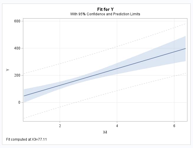
These statements create data set, CHK, containing two settings of x4 that are one unit apart and at the mean of x3. The SCORE statement produces predicted values for these two points. PROC MEANS displays the estimates at the two points and the RANGE option computes their difference. The EFFECTPLOT statement displays the fitted model as a function of x4 while holding x3 at its mean (77.11):
     data chk;
        x3=77.111111;
        do x4=2,3; output; end;
        run;
     proc plm restore=SurgReg;
        effectplot fit(x=x4);
        score data=chk out=chkout predicted=pred;
        run;
     proc means data=chkout min max range;
        var pred;
        run;
The plot of the fitted model at the mean x3 is shown below. The PROC MEANS results provide the estimated means at x4=2 and x4=3. It also gives a point estimate of the difference in these means, 61.8:
 |
|||||||||
|
|||||||||
Using the Margins Macro
In the Margins macro, the above model is specified using data=, response=, and model=. The macro uses the GENMOD procedure to fit the specified model. The continuous marginal effect is computed by specifying effect=x4 in the Margins macro. To compute it with x3 fixed at its mean, specify mean=x3 or options=atmeans as done in the first Margins call below. If neither is specified, the marginal effect is an average over the observations using their actual x3 values as done in the second Margins call. Confidence limits are requested with options=cl:
   %Margins(data=surg, response=y, model=x3|x4,
          effect=x4, mean=x3, options=cl)
   %Margins(data=surg, response=y, model=x3|x4,
          effect=x4, options=cl)
The results include the fitted model (not shown). The estimated continuous marginal effect is 61.8 with 95% confidence interval (39.7, 83.9). The marginal effect estimate from the second approach is the same as from the first for this model since averaging over the observations using the actual x3 values is the same as using the x3 mean. Note that, in general, the marginal effect for x4 would depend on the setting of both x3 and x4 where it is computed. But the fitted model at any x3 value is a straight line and a line drawn tangent to it at any value of x4 is the same straight line. So, the marginal effect (slope of the tangent line) does not change with x4:
 |
To compute the categorical marginal effect, first specify the desired two settings of x4 as two observations in a data set (MDAT), which is then specified in margindata=. The predictive margins for x4 at the mean of x3 are requested using margins=x4 and mean=x3. Alternatively, they can be computed as averages using the actual x3 values if omitted. The diff and cl options request the difference in the two predictive margins and its confidence interval. The difference is the categorical marginal effect over the two specified levels of x4. The reverse option requests the (x4=3) - (x4=2) difference rather than the default, which is in the opposite order. This provides the estimate of increasing x4 from x4=2 to x4=3:
    data mdat;
      do x4=2,3;
        output;
      end;
      run;
    %Margins(data=surg, response=y, model=x3|x4,
             margins=x4, margindata=mdat, mean=x3,
             options=diff reverse cl)
The results include the fitted model (not shown), the x3 mean value that was used, the response means at the two settings of x4, and their difference, 61.8, which agrees with the point estimate above. Notice that the categorical and continuous marginal effects are identical in this case because the fitted model at fixed x3 is a straight line, as shown above, and a line drawn tangent to it at any x4 value would be the same straight line. As a result, both slopes are the same and therefore the two marginal effects are the same:
|
Using the HAZARDRATIO and ESTIMATE Statements
To determine the coefficients needed in an ESTIMATE statement, fit the model in PROC PHREG and include the HAZARDRATIO statement. Note that if the response contains any negative values, those observations are omitted by PROC PHREG. The same observations should be included in the PHREG analysis as when fitting the model using the intended modeling procedure. Since the determination of contrast coefficients does not depend on the actual response values, you can use any positive values. It is easiest to simply generate a variable of random positive values for any nonmissing values in the original response. In the DATA step that follows, a variable, RAND, is created that contains a random value between 0 and 1 for any nonmissing value of Y.
As mentioned above, you should ignore PROC PHREG output except the Hazard Ratios table. The ODS SELECT statement limits the displayed results to this one table. By default, the E option in the HAZARDRATIO statement adds to this table the contrast coefficients that estimate the effect of a one-unit increase in x4 at the mean of the interacting continuous variable, x3:
      data surg;
        set surg;
        rand=y;
        if y ne . then rand=ranuni(2342);
        run;
      proc phreg data=surg;
        model rand = x3|x4;
        hazardratio x4 / e;
        ods select hazardratios;
        run;
The contrast coefficients are shown in the Hazard Ratios table:
|
|||||||||||||||||||||
To estimate the effect of changing the variable of interest by more or less than one unit, specify the desired unit or units of change in the UNITS= option in the HAZARDRATIO statement. Also, to estimate the effect of the change at specific values of the interacting variable(s), specify the AT option. For example, to estimate the effects of changing x4 by 1.5 and 2 units at several settings of x3 (50, 75, and 100), the following HAZARDRATIO statement provides the coefficients for use in subsequent ESTIMATE or CONTRAST statements:
hazardratio x4 / units=1.5 2 at (x3=50 75 100) e;
The effect of a unit increase in x4 with x3 fixed at its mean can now be assessed in the fit of the actual model using these coefficients in an ESTIMATE statement in the GLM procedure or other appropriate procedure. Note that effects with zero coefficient can be omitted. It is a good idea to include the E option in the ESTIMATE statement to verify that the coefficients are the same as provided by PROC PHREG. The fitted model is saved in an item store named RegMod for later use:
      proc glm data=surg;
        model y=x3|x4;
        estimate 'x4+1 at mean(x3)' x4 1 x3*x4 77.111111 / e;
        store SurgReg;
        run; quit;
The ESTIMATE statement results show that the effect of increasing x4 by one unit with x3 at its mean is 61.8. Note that this agrees with the marginal effect estimates obtained from the Margins macro and the point estimate using predicted values. The standard errors here and from the Margins macro differ slightly because different computational methods are used. The table of coefficients verifies that the coefficients were the same as shown earlier by PHREG:
|
||||||||||||||||||||||
Continuous-Categorical Interaction in a Log-Linked Model
When the interacting variable is categorical rather than continuous, it is the effect of changing the continuous variable at each level of the categorical variable that is of interest.
This example fits a Poisson model to data from Long (1997) that models the numbers of articles published by scientists (ART) as a function of various predictors. In this model, the predictors are the prestige of the scientists' PhD program (PHD) and the number of young children that they have (KID5). Of interest is estimating the effect of an increase in program prestige on the number of published articles. The data are available in the SAS/ETS® Sample Library in example programs for the COUNTREG procedure.
Two estimates of the effect of prestige can be obtained. Since the model involves the log link function, the ESTIMATE statement can give only the multiplicative effect by estimating the ratio of the response means, when comparing two populations that differ by a fixed number of units of prestige. The Margins macro can estimate the additive effect by estimating the difference in response means for the same two populations.
Using Predicted Values to Estimate the Difference and Ratio of Response Means
As done in the previous example, the following statements estimate the model, plot it, and estimate the response mean at desired predictor values. Data set CHK is created that contains the two settings of prestige that are two units apart and with no children. The ILINK option is specified in the EFFECTPLOT statement to plot the predicted mean response on the vertical axis rather than the default log of the response mean (the linear predictor). The ILINK option is also used in the SCORE statement to obtain predicted mean article counts. Point estimates of the difference and ratio of means are obtained using the estimated means:
proc genmod data=long97data;
class kid5 / param=glm;
model art = phd|kid5 / dist=poisson link=log;
store PhdMod;
run;
data chk;
kid5=0;
do phd=2,4;
output;
end;
run;
proc plm restore=PhdMod;
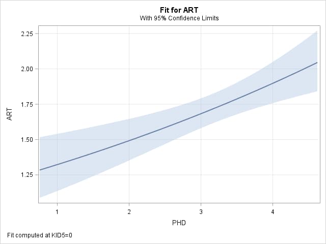
effectplot fit(x=phd) / at(kid5='0') ilink;
score data=chk out=chkout predicted=pred / ilink;
run;
proc means data=chkout min max range;
var pred;
run;
The resulting plot and range value from PROC MEANS show that the estimated increase in response mean for an increase in two units of prestige with no children is 0.4063. Also, the multiplicative effect of increasing prestige by two units as measured by the ratio of means is 1.898 / 1.492 = 1.272. That is, the mean number of articles is estimated to increase by a factor of 1.272 when increasing prestige by two units:
|
|||||||||
Using the Margins Macro to Estimate the Difference in Response Means
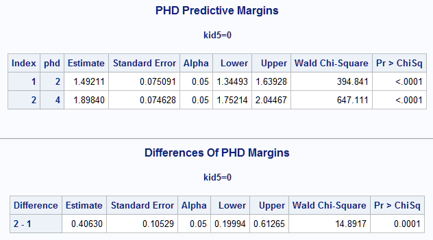
The difference in response means can also be computed as the categorical marginal effect of prestige using the Margins macro (SAS Note 63038). The macro fits the model and estimates the means and their difference. Neither PROC GENMOD nor PROC PHREG is needed for this approach. The two prestige levels to estimate and compare are specified in two observations specified in data set MDAT. The means are estimated and compared for the case of no children as indicated by the one observation in data set ADAT. The same model as above is specified in the Margins macro using data=, class=, response=, model=, and dist=. The predictive margins for the two prestige levels are requested using margins= and margindata=. This is estimated in the no children population using at= and atdata=. The diff and cl options request the difference in the two predictive margins and its confidence interval. This is the categorical marginal effect over these two specified levels of prestige. The reverse option requests the (PHD=4) - (PHD=2) difference rather than the default, which is in the opposite order:
    data mdat;
       do phd=2,4;
         output;
       end;
       run;
    data adat;
       kid5=0;
       run;
    %Margins(data=long97data, class=kid5, response=art, model=phd|kid5, dist=poisson,
             margins=phd, margindata=mdat, at=kid5, atdata=adat, options=diff reverse cl)
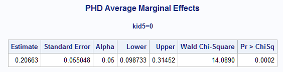
The Margins macro also provides the estimated means at each level of prestige as well as their difference:
 |
Getting the Equivalent of LSMEANS for a Continuous Variable
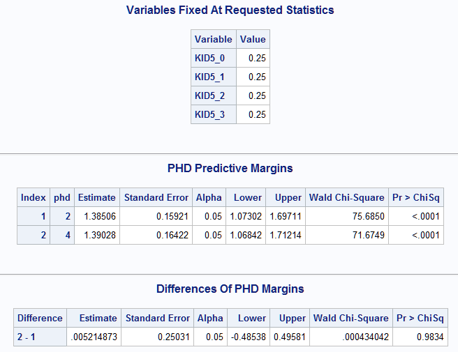
The equivalent of the estimate that the LSMEANS statement would give if it could operate on a continuous variable can also be obtained. Note that the LSMEANS statement for a categorical variable or model effect simply estimates particular linear combinations of the model parameters, which can be adjusted somewhat using available options in that statement. This implies that it can estimate response means by setting all of the model variables to certain fixed values as reflected by the coefficients that it uses. By default, when computing an LS-mean, the coefficient for any continuous covariate is fixed at its mean, and for a categorical covariate, the coefficients are equal proportions. This can effectively be done in the Margins macro as above but omitting at= and atdata= and also specifying all continuous covariates in mean= and all categorical covariates in balanced=. For this model with only a categorical covariate, balanced=kid5 is specified:
    %Margins(data=long97data, class=kid5, response=art, model=phd|kid5, dist=poisson,
             margins=phd, margindata=mdat, balanced=kid5, options=diff reverse cl)
Because balanced=kid5 is specified, the predictive margins are averaged over the balanced levels of KID5 rather than at KID5=0 (no children). When averaged over the numbers of children, the difference in response means is very small (0.005). Note that including the OM option in the LSMEANS statement changes the coefficients that it uses for categorical covariates to be proportional to the observed levels. The equivalent can be done in the Margins macro by specifying atmeans in options= and omitting balanced=, mean=, or at= (not shown):
 |
Using the Margins Macro to Estimate the Instantaneous Rate of Change
The continuous marginal effect of prestige can be computed at any setting of the model predictors. At any given setting, it tells you the instantaneous rate of change in the response mean at that point. The following statements use the Margins macro to compute the continuous marginal effect at several prestige values (PHD=1, 2, 3, 4) with no children (KID5=0):
    data adat;
       kid5=0;
       do phd=1 to 4;
         output;
       end;
       run;
    %Margins(data=long97data, class=kid5, response=art, model=phd|kid5, dist=poisson,
             effect=phd, at=kid5 phd, atdata=adat, options=cl noprintbyat)
Notice that the instantaneous change in the mean number of published articles accelerates as prestige increases. The slope of the tangent lines drawn at these points increases:
 |
An overall average slope for prestige in the no children population can be obtained by averaging over all of the observation-specific marginal effects that are computed using each observed prestige value. This average slope is obtained by simply removing phd from at=:
    %Margins(data=long97data, class=kid5, response=art, model=phd|kid5, dist=poisson,
             effect=phd, at=kid5, atdata=adat, options=cl)
 |
Effect of Continuous Predictor in Model with Multiple interactions
Consider the automobile fuel efficiency data analyzed in the Getting Started section of the ADAPTIVEREG procedure documentation, which provides a link to the data. Suppose that a model is fit involving four variables including both categorical and continuous variables. The model includes higher-order terms as well as main effects. Of particular interest is to estimate the effect of increasing model years on the fuel efficiency (miles per gallon) of domestic cars. Other predictors in the model are the horsepower rating, number of cylinders, and origin of manufacture. Model year is involved in interactions with a categorical variable and a continuous variable and appears both as linear and quadratic effects.
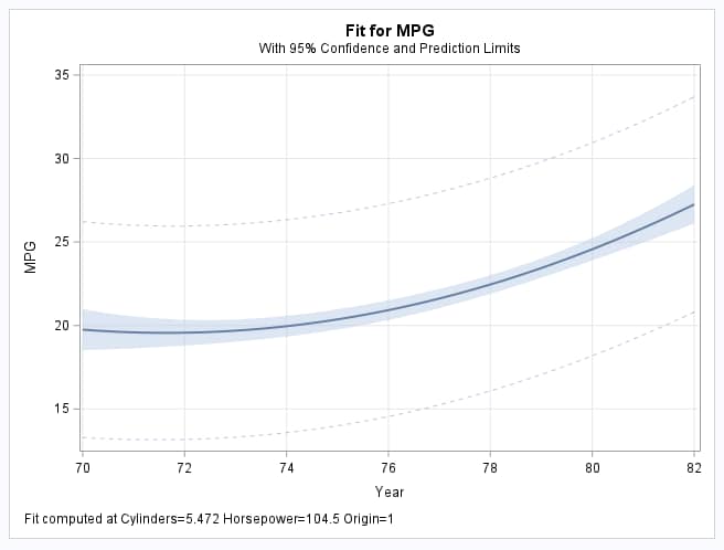
These statements fit the model, plot the estimated efficiency for domestic cars (ORIGIN=1) as a function of model year with other variables held fixed their means, and save the fitted model for later use:
    proc orthoreg data=autompg;
       class origin;
       model mpg = cylinders year|year|horsepower@2 year|origin horsepower*origin;
       effectplot fit(x=year) / at (origin='1');
       store AutoMod;
       run;
As shown in the plot, increasing model year results in increasing fuel efficiency in domestic cars and the increase accelerates in later model years:
 |
Using Predicted Values
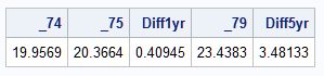
These statements obtain point estimates of the miles per gallon for each of the model years 74, 75, and 79 for domestic cars with horsepower and cylinders held at their means. The one- and five-year differences are also computed and displayed:
    data chk;
       origin=1; cylinders=5.472; horsepower=104.5;
       do year=74,75,79;
         output;
       end;
       run;
    proc plm restore=AutoMod;
       score data=chk out=chkout predicted=pred;
       run;
    proc transpose data=chkout out=chkout2;
       var pred; id year;
       run;
    data chkout2; set chkout2;
       Diff1yr=_75-_74;
       Diff5yr=_79-_74;
       run;
    proc print data=chkout2 noobs;
       var _74 _75 Diff1yr _79 Diff5yr;
       run;
The effect of a one model year increase starting at year 74 is observed to be 0.41 and 3.48 for an increase of three years. These changes are consistent with the above plot of the model:
 |
Using the Margins Macro to Estimate the Difference in Response Means
As with the first example above, the Margins macro can estimate the change in efficiency for increasing model year using either categorical or continuous marginal effects. Beginning with the categorical marginal effect, the MDAT data set created below specifies three model years, 74, 75, and 79, for assessing the effect of an increase of 1 year and 5 years. These comparisons will be done for domestic cars (ORIGIN=1) as specified in data set ADAT. In the Margins macro, the above model is specified in response=, class=, and model=. The means for the three model years for domestic cars are requested in margins=, margindata=, at=, and atdata=. Comparisons among the years, with confidence intervals, are requested with the diff, reverse, and cl options:
    data mdat;
       do year=74,75,79;
         output;
       end;
       run;
    data adat;
       origin=1;
       run;
    %Margins(data=autompg, response=mpg, class=origin,
             model=cylinders year|year|horsepower@2 year|origin horsepower*origin,
             margins=year, margindata=mdat, at=origin, atdata=adat,
             options=diff reverse cl)
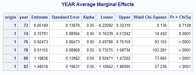
The estimated margins for each year and their differences are given in the Predictive Margins table and Differences of Margins tables. For domestic cars, a one model year increase results in an increase of 0.41 miles per gallon with 95% confidence interval (0.25, 0.56). Over five years, the increase is 3.48 miles per gallon with 95% confidence interval (2.83, 4.13). These increases are computed as the difference, between years, in the averages of predicted values using the actual values for horsepower and cylinders:
 |
Getting the Equivalent of LSMEANS for a Continuous Variable
The equivalent of LSMEANS estimates and their differences can be obtained as described in the previous example. The following shows the appropriate Margins macro calls (results not shown). The LSMEANS default fixes horsepower and cylinders at their means and origin at equal proportions:
    %Margins(data=autompg, response=mpg, class=origin,
             model=cylinders year|year|horsepower@2 year|origin horsepower*origin,
             margins=year, margindata=mdat, balanced=origin, mean=horsepower cylinders,
             options=diff reverse cl)
Equivalents to LSMEANS with the OM option does the same but uses the observed proportions for origin:
    %Margins(data=autompg, response=mpg, class=origin,
             model=cylinders year|year|horsepower@2 year|origin horsepower*origin,
             margins=year, margindata=mdat, options=atmeans diff reverse cl)
Using the Margins Macro to Estimate the Instantaneous Rate of Change
The instantaneous rate of change in efficiency at specific years can also be obtained. The following statements estimate the continuous marginal effect for domestic cars at model years between 72 and 82:
    data adat;
       origin=1;
       do year=72 to 82 by 2;
         output;
       end;
       run;
    %Margins(data=autompg, response=mpg, class=origin,
             model=cylinders year|year|horsepower@2 year|origin horsepower*origin,
             effect=year, at=origin year, atdata=adat, options=cl noprintbyat)
Consistent with the plot of the fitted model above, the rate of fuel efficiency increase itself increases across the model years:
 |
If the increasing rate of change is ignored, an average rate of change for domestic cars can be obtained by removing YEAR from at=:
    %Margins(data=autompg, response=mpg, class=origin,
             model=cylinders year|year|horsepower@2 year|origin horsepower*origin,
             effect=year, at=origin, atdata=adat, options=cl)
The average rate of change over the model years for domestic cars is found to be 0.62 miles per gallon:
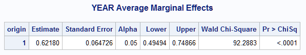 |
Using the HAZARDRATIO and ESTIMATE Statements
Since this is an ordinary regression model that uses the identity link, the HAZARDRATIO statement can be used in PHREG to determine the contrast coefficients that estimate the effect of increasing model year by specific amounts while holding the other model predictors at specific values.
These statements produce the coefficients needed to assess the effect of increasing model year by 1 and 5 years, starting at year 74, in domestic cars with horsepower and cylinders fixed at their means. Since MPG is a nonnegative variable, the variable can be used directly in PROC PHREG:
    proc phreg data=autompg;
       class origin / param=glm;
       model mpg = cylinders year|year|horsepower@2 year|origin horsepower*origin;
       hazardratio year / units=1 at (origin='1' year=74) e;
       hazardratio year / units=5 at (origin='1' year=74) e;
       ods select hazardratios;
       run;
The contrast coefficients appear in the Hazard Ratios tables:
|
||||||||||||||||||||||||||||||||||||||||||||||||||||||||||||||||||||||||||||||||||||||||||||||||||||||||||||
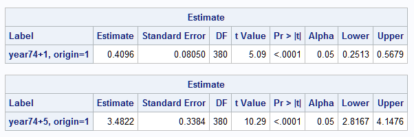
The coefficients can then be used in ESTIMATE statements in PROC PLM to produce the effect estimates:
    proc plm restore=AutoMod;
       estimate 'year74+1, origin=1' year 1 year*year 149 year*horsepower 104.469388 year*origin 1 / cl;
       estimate 'year74+5, origin=1' year 5 year*year 765 year*horsepower 522.346939 year*origin 5 / cl;
       run;
Since the identity link function is used in this model (that is, the mean is modeled directly, rather than a function of it), the estimates for one- and five-year increases match the categorical marginal effects from the Margins macro above. As noted in the first example, these standard errors and those from the Margins macro differ slightly because different computational methods are used:
 |
Models Involving Constructed Effects Such as Splines
The HAZARDRATIO statement is particularly useful in complex models using the identity link such as those that involve constructed effects. Several types of constructed effects are available with the EFFECT statement that can be used in many modeling procedures. Splines are one type of constructed effect commonly used when the association of a continuous predictor on the response is complex and unknown. The spline is a very flexible function that can accommodate complex relationships between predictor and response.
The following example uses the diabetes data in the Getting Started section of the GAM procedure's documentation. The data are available in the SAS/STAT® Sample Library in example programs for the GAM procedure. The model assesses the association of subject age (AGE) and a measure of acidity (BaseDeficit) on the log of the serum C-peptide level (logCP). A natural cubic spline is applied to BaseDeficit to allow for a complex association of that variable with the response. Both linear and quadratic effects of AGE are included in the model and the BaseDeficit spline is allowed to interact with both AGE effects. The EFFECT and MODEL statements below specify this model.
Note that the Margins macro cannot be used since the macro does not support models that involve constructed effects such as splines. The method using the HAZARDRATIO and ESTIMATE statements is shown. For generalized linear models that include spline effects but do not use the identity link, another approach using the NLMeans macro can be used to estimate and plot difference or ratios of response means over a continuous variable as is illustrated in SAS Note 70221:
After fitting the model, it is of interest to estimate the effect of increasing BaseDeficit by one unit, from -10 to -9, when AGE is fixed at 10. The following statements define the model and include a HAZARDRATIO statement to produce the coefficients needed to estimate this effect:
      proc phreg data=diabetes;
         effect s = spline(BaseDeficit / naturalcubic);
         model logCP = s|age|age;
         hazardratio BaseDeficit / at (BaseDeficit=-10 age=10) e;
         ods select hazardratios;
         run;
Following are the coefficients produced by the HAZARDRATIO statement:
|
|||||||||||||||||||||||||||||||||||||||||||||
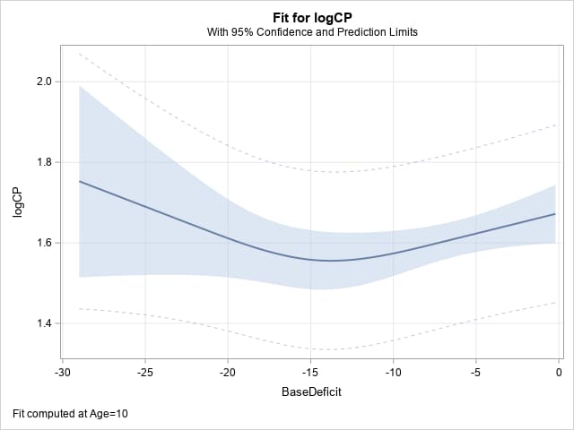
The model can now be fit using PROC ORTHOREG and the effect estimated using the coefficients provided by the HAZARDRATIO statement. The EFFECTPLOT statement below is included to visualize the effect of interest. It requests a plot of the predicted response against BaseDeficit when AGE is fixed at 10. The fitted model is also saved by the STORE statement in an item store named RegMod:
      proc orthoreg data=diabetes;
         effect s = spline(BaseDeficit / naturalcubic);
         model logCP = s|age|age;
         estimate 'BD+1 @BD=-10,age=10'
                  s 0 1 20.663889   s*age 0 10 206.638889
                  s*age*age 0 100 2066.388889 / cl e;
         effectplot fit(x=BaseDeficit) / at (age=10);
         store RegMod;
         run;
The results from the ESTIMATE and EFFECTPLOT statements are shown below. The estimated effect of increasing BaseDeficit by one unit at -10 when AGE=10 is about 0.009. The effect of larger changes could be obtained by including the UNITS= option in the HAZARDRATIO statement:
 |
|||||||||||||||||||||||||||
To check the effect estimated by the ESTIMATE statement, the following statements evaluate the fitted model at two BaseDeficit settings, -10 and -9, with AGE fixed at 10. The two settings are created in data CHK and predicted values are computed for each using the SCORE statement in PROC PLM. PROC MEANS displays the estimates at the two points and computes their difference:
      data chk;
         age=10;
         do BaseDeficit=-10, -9;
           output;
         end;
         run;
      proc plm restore=RegMod;
         score data=chk out=chkout predicted=pred;
         run;
      proc means data=chkout min max range;
        var pred;
        run;
The predicted values are shown below. The difference (Range) is equal to the 0.009 estimate produced by the ESTIMATE statement:
|
|||||||||
___________
References
Long, J. S. (1997). Regression Models for Categorical and Limited Dependent Variables. Thousand Oaks, CA: Sage Publications.
Operating System and Release Information
| Product Family | Product | System | SAS Release | |
| Reported | Fixed* | |||
| SAS System | SAS/STAT | z/OS | ||
| z/OS 64-bit | ||||
| OpenVMS VAX | ||||
| Microsoft® Windows® for 64-Bit Itanium-based Systems | ||||
| Microsoft Windows Server 2003 Datacenter 64-bit Edition | ||||
| Microsoft Windows Server 2003 Enterprise 64-bit Edition | ||||
| Microsoft Windows XP 64-bit Edition | ||||
| Microsoft® Windows® for x64 | ||||
| OS/2 | ||||
| Microsoft Windows 8 Enterprise 32-bit | ||||
| Microsoft Windows 8 Enterprise x64 | ||||
| Microsoft Windows 8 Pro 32-bit | ||||
| Microsoft Windows 8 Pro x64 | ||||
| Microsoft Windows 8.1 Enterprise 32-bit | ||||
| Microsoft Windows 8.1 Enterprise x64 | ||||
| Microsoft Windows 8.1 Pro 32-bit | ||||
| Microsoft Windows 8.1 Pro x64 | ||||
| Microsoft Windows 10 | ||||
| Microsoft Windows 95/98 | ||||
| Microsoft Windows 2000 Advanced Server | ||||
| Microsoft Windows 2000 Datacenter Server | ||||
| Microsoft Windows 2000 Server | ||||
| Microsoft Windows 2000 Professional | ||||
| Microsoft Windows NT Workstation | ||||
| Microsoft Windows Server 2003 Datacenter Edition | ||||
| Microsoft Windows Server 2003 Enterprise Edition | ||||
| Microsoft Windows Server 2003 Standard Edition | ||||
| Microsoft Windows Server 2003 for x64 | ||||
| Microsoft Windows Server 2008 | ||||
| Microsoft Windows Server 2008 R2 | ||||
| Microsoft Windows Server 2008 for x64 | ||||
| Microsoft Windows Server 2012 Datacenter | ||||
| Microsoft Windows Server 2012 R2 Datacenter | ||||
| Microsoft Windows Server 2012 R2 Std | ||||
| Microsoft Windows Server 2012 Std | ||||
| Microsoft Windows Server 2016 | ||||
| Microsoft Windows Server 2019 | ||||
| Microsoft Windows XP Professional | ||||
| Windows 7 Enterprise 32 bit | ||||
| Windows 7 Enterprise x64 | ||||
| Windows 7 Home Premium 32 bit | ||||
| Windows 7 Home Premium x64 | ||||
| Windows 7 Professional 32 bit | ||||
| Windows 7 Professional x64 | ||||
| Windows 7 Ultimate 32 bit | ||||
| Windows 7 Ultimate x64 | ||||
| Windows Millennium Edition (Me) | ||||
| Windows Vista | ||||
| Windows Vista for x64 | ||||
| 64-bit Enabled AIX | ||||
| 64-bit Enabled HP-UX | ||||
| 64-bit Enabled Solaris | ||||
| ABI+ for Intel Architecture | ||||
| AIX | ||||
| HP-UX | ||||
| HP-UX IPF | ||||
| IRIX | ||||
| Linux | ||||
| Linux for x64 | ||||
| Linux on Itanium | ||||
| OpenVMS Alpha | ||||
| OpenVMS on HP Integrity | ||||
| Solaris | ||||
| Solaris for x64 | ||||
| Tru64 UNIX | ||||
| Type: | Usage Note |
| Priority: | |
| Topic: | Analytics ==> Regression SAS Reference ==> Procedures ==> PHREG SAS Reference ==> Macro |
| Date Modified: | 2023-07-07 16:52:24 |
| Date Created: | 2020-12-02 15:49:08 |