Generate multivariate binary data with given means and correlation matrix

Contents:

Purpose / History / Requirements / Usage / Details / Limitations / References

 

PURPOSE:

The RanMBin macro generates values from multiple binary variables with specified means and correlation matrix. It creates an output data set with the specified number of observations and arranged either in wide or long format. Exchangeable and autoregressive AR(1) correlation structures are supported as well as unstructured correlation matrices. Banded correlation structures with autoregressive, power-decaying correlations are also easily handled.

HISTORY:

The version of the RanMBin macro that you are using is displayed when you specify version (or any string) as the first argument. For example:

    %RanMBin(version, )

The RanMBin macro always attempts to check for a later version of itself. If it is unable to do this (such as if there is no active internet connection available), the macro will issue the following message:

   NOTE: Unable to check for newer version

The computations performed by the macro are not affected by the appearance of this message.

Version	Update Notes
1.1	Corrected Prentice constraint computation
1.0	Initial coding

REQUIREMENTS:

Only Base SAS^® is required.

USAGE:

Follow the instructions on the Downloads tab of this sample to save the RanMBin macro definition. Replace the text within quotation marks in the following statement with the location of the RanMBin macro definition file on your system. In your SAS program or in the SAS editor window, specify this statement to define the RanMBin macro and make it available for use:

   %inc "<location of your file containing the RanMBin macro>";

Following this statement, you can call the RanMBin macro. See the Results tab for examples.

The following parameters are required when using the RanMBin macro:

means=value-list , or
inmeans=data-set

Either means= or inmeans= is required to specify the number of binary variables, m, to be created and their means. If means= and inmeans= are both specified, inmeans= is ignored.

If inmeans= is specified, the first observation in the data set is read. The number of numeric variables in the data set determines the number of binary variables to be created. The values in all numeric variables are used as means of the desired binary variables. The values in the variables must be real numbers between 0 and 1. The names of the numeric variables in the data set is not restricted.

If means= is specified, value-list is a space-separated list of real numbers between 0 and 1. Additionally, any value in the list can be integer*value, where integer is a positive integer to specify that value should be replicated integer times. For example, means=0.4 2*0.1 3*0.15 is equivalent to means=0.4 0.1 0.1 0.15 0.15 0.15.

 

exch=value , or
ar=value , or
incorr=data-set

One of exch=, ar=, or incorr= must be specified to determine the correlations among the m binary variables to be created. Specify exch= to create a correlation matrix with exchangeable structure in which every pair of variables has the specified correlation value. An autoregressive structure is created by specifying ar=. See k= for how it modifies that structure. If exch= or ar= is specified, value must be a real number between 0 and 1. If incorr= is specified, the data set must have exactly m numeric variables. The names of the numeric variables in the data set are not restricted. The observations in the data set must contain the desired correlation matrix with positive correlations. The i^th row and column in the data set should contain the correlations corresponding with the i^th mean. Only the values in the upper triangle above the main diagonal are read. Values on and below the main diagonal are ignored.

 

The following parameters are optional:

out=data-set

Specifies the name of the data set to be created that contains the generated random variables. The variables, the number of observations, and the shape of the data set depend on outshape=. See the descriptions of outshape= and n= for details. If omitted, out=Mbin.

outshape=wide|long

Specifies the shape and structure of the out= data set. If outshape=wide, each observation contains one set of m random values (either 0 or 1) for the m binary variables named Y1-Ym. The data set contains n observations as specified by n=. If outshape=long, each set of m random values creates m observations and all random values are placed in a single binary variable named Y. The data set contains nm observations. The probability that a random value equals 1 is equal to the corresponding mean as specified in means= or inmeans=. A numeric variable identifying the separate sets of generated random values is included in the data set. It is named ID by default with values 1, 2, and so on. If outshape=long, an additional variable is added to identify the binary variable within each generated set. It is named SubID by default with values 1, 2, ... , m in each set. If omitted, outshape=wide.

n=n

Specifies the number of sets of random values to create in the out= data set. Each set contains m random values for the m binary variables with the specified means and correlation matrix. Each value is either 0 or 1. If omitted, n=100.

subject=variable-name

Specifies the name of the numeric variable in the out= data set that identifies each set of m generated random values. See the description of outshape= for details. If omitted, subject=ID.

within=variable-name

Specifies the name of the numeric variable in the out= data set that identifies the binary variable within each set of m generated random values when outshape=long. within= is ignored if outshape=wide. See the description of outshape= for details. If omitted, within=SubID.

k=k

Specifies the number of bands, k=1, 2, ..., m-1, parallel to the main diagonal that will contain non-zero correlation values. All correlations in bands beyond the k^th band will be set to zero. k= can be specified with ar= or incorr=. When specified with ar=α, the correlation matrix has value α^k for all elements in the k^th band and zero for all bands beyond k. If specified with incorr=, any non-zero correlations specified beyond the k^th band are ignored and set to zero. If omitted, k=m-1.

seed=number

Specifies an integer used to start the generation of random values. If you do not specify a seed, or if you specify a value less than or equal to zero, the seed is by default generated from reading the time of day from the computer's clock. If omitted, seed=0.

DETAILS:

Wei et al. (2020) present algorithms that "generate high-dimensional binary data with specified correlation structures and unequal probabilities." The RanMBin macro implements three of these algorithms and can generate random values from m binary variables that have specified means (means= or inmeans=) and a correlation matrix with exchangeable (exch=) , autoregressive AR(1) (ar=), or banded power-decaying structures (ar= with k=). Random values can also be generated when the correlation matrix is fully unstructured (incorr=).

The macro creates an output data set (out=) with n observations (n=) and random values in variables Y1, Y2, ..., Ym if a wide data set structure (outshape=wide) is selected, or nm observations if a long structure (outshape=long) is desired. The output data set contains a variable (subject=) that numbers the observations in the wide format. In the long format, each generated set of random values for the m variables creates m output observations that are placed in a single variable, Y. Also included is a variable (subject=) that identifies the set of random values and another variable (within=) that identifies the random variable in the set associated with each observation. Reproducible sets of random values can be obtained by specifying a seed (seed=).

Errors and constraints

As noted by Wei et al. (2020) and in "Generalized Estimating Equations" in the Details section of the GENMOD documentation, there are natural restrictions on the correlations among binary variables. Prentice (1988) developed formulas expressing the constraints and these are presented by Wei et al. The macro checks the specified means and correlations to verify that the Prentice constraints are satisfied. Any violations are displayed. When violations occur, changes to the specified means and/or correlations can be made in a subsequent run of the macro. In addition, the algorithm used when incorr= or k= is specified can fail when computation of a binomial probability results in an invalid value. A note is displayed in the log when either this failure or violations of the Prentice constraints occurs.

The macro does not create any displayed output unless violations of the Prentice constraints are detected as noted above.

The RanMBin macro can be used to simulate multivariate binary data for many situations such as when a binary response is measured over time or under many conditions. Such data is often modeled using a Generalized Estimating Equations (GEE) or random effects model such as available in the GEE, GENMOD, and GLIMMIX procedures. The correlation structures available in the macro are commonly used in GEE models.

Multiple means vectors and/or correlation matrices

While the RanMBin macro does not directly support random value generation for multiple mean vectors and/or correlation matrices, this can be done using the RunBY macro. With it, you can run the RanMBin macro repeatedly for each mean vector in the inmeans= data set and/or each correlation matrix in the incorr= data set. See the RunBY macro documentation for details on its use. Also see the example titled "Multiple mean vectors" on the Results tab above.

LIMITATIONS:

All correlations must be positive.

REFERENCES:

Prentice, R. L. (1988), "Correlated Binary Regression with Covariates Specific to Each Binary Observation," Biometrics, 44, 1033-1048.

Wei J., Shuang S., Lin H., and Hongyu Z. (2020), "A Set of Efficient Methods to Generate High-Dimensional Binary Data With Specified Correlation Structures," The American Statistician, DOI: 10.1080/00031305.2020.1816213.

 

---

These sample files and code examples are provided by SAS Institute Inc. "as is" without warranty of any kind, either express or implied, including but not limited to the implied warranties of merchantability and fitness for a particular purpose. Recipients acknowledge and agree that SAS Institute shall not be liable for any damages whatsoever arising out of their use of this material. In addition, SAS Institute will provide no support for the materials contained herein.

---

---

These sample files and code examples are provided by SAS Institute Inc. "as is" without warranty of any kind, either express or implied, including but not limited to the implied warranties of merchantability and fitness for a particular purpose. Recipients acknowledge and agree that SAS Institute shall not be liable for any damages whatsoever arising out of their use of this material. In addition, SAS Institute will provide no support for the materials contained herein.

In the examples below, a seed value is specified in the seed= parameter of the RanMBin macro so that the same random values can be produced and the numeric results shown can be reproduced.

Note that since the macro produces a finite number of realizations of the specified binary distributions, the specified means and correlation matrix can never be exactly replicated by the generated data. However, as the number of observations, n, increases, the means and correlations come arbitrarily close to their specified values.

EXAMPLE 1: Exchangeable correlation structure

The following call of the RanMBin macro produces 100,000 observations of three binary variables with means 0.1, 0.4, and 0.5. The PROC PRINT step displays the first ten observations of the default Mbin data set.

    %RanMBin(means=.1 .4 .5, exch=.1, n=100000, seed=38473)
    proc print data=Mbin(obs=10) noobs;
      id id;
      run;

ID Y1 Y2 Y3 1 0 1 0 2 0 0 0 3 0 0 1 4 0 0 1 5 0 0 0 6 0 0 1 7 0 0 0 8 0 0 1 9 0 0 0 10 0 1 0

The exchangeable correlation structure has a common correlation among all pairs of variables. In this example, the common correlation is 0.1. The results from PROC CORR shows that the generated random variables have the specified means and correlation structure.

    proc corr data=mbin;
      var y:;
      run;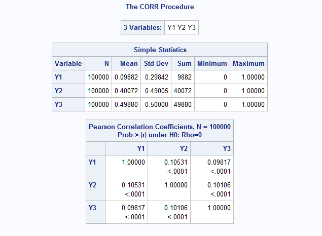

EXAMPLE 2: Autoregressive AR(1) correlation structure

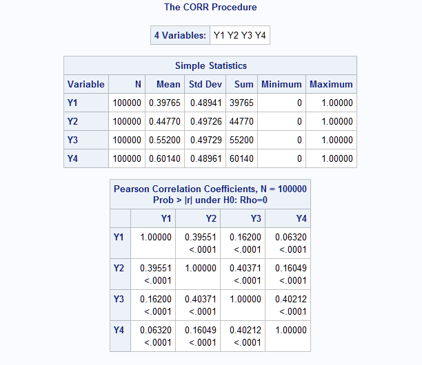
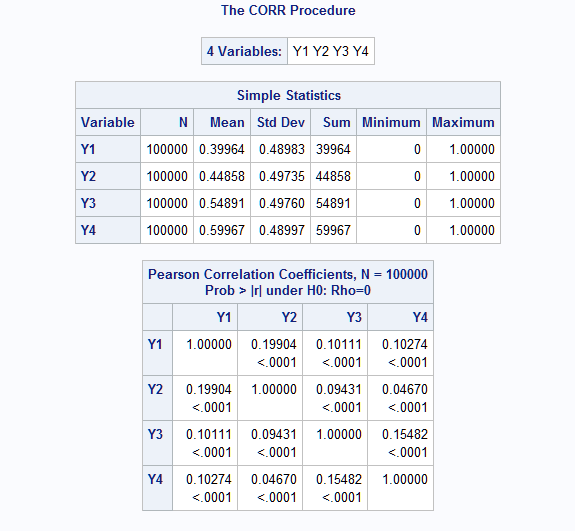
This macro call generates m=4 binary variables with the means as specified in means=. The AR(1) correlation structure is such that the correlations in the first band next to the main diagonal all equal 0.4. In the second band, the correlations equal 0.4² = 0.16. The third (m-1 = 3) and final band has correlations 0.4³ = 0.064.

    %RanMBin(means=.4 .45 .55 .6, ar=.4, n=100000, seed=38473)
    proc corr data=mbin;
      var y:;
      run;

The results from PROC CORR show that the mean and correlation values are all closely reproduced by the generated data.

EXAMPLE 3: Banded power-decaying correlation structure

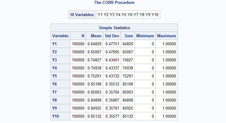
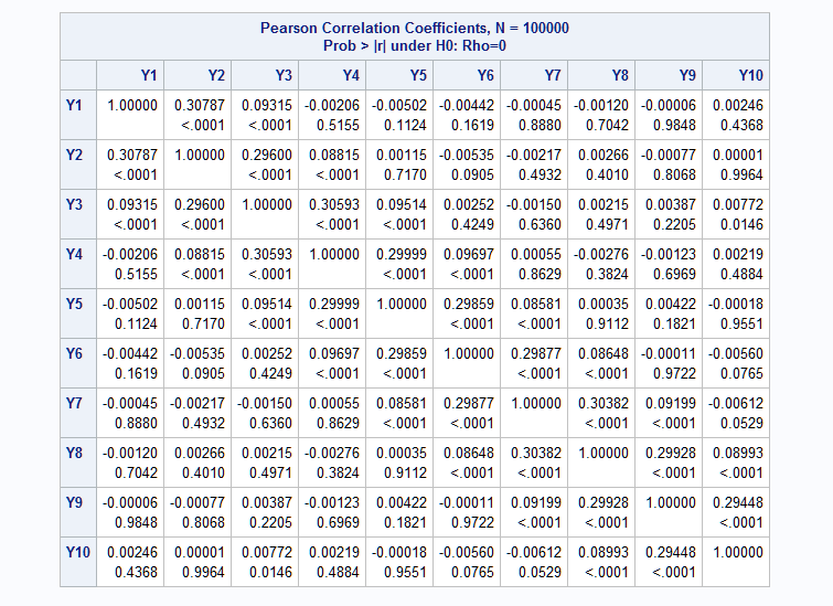
The following macro call generates ten binary variables. The means are specified using asterisks to replicate values. The specification in this example is equivalent to means=.65 .65 .75 .75 .75 .85 .85 .85 .85 .85. The ar=.3 k=2 specification creates a correlation structure with only two bands of non-zero correlations and with the non-zero correlations decaying from the first to the second band using the band number as the power on 0.3. So, the correlations in the first band equal 0.3¹ = 0.3. In the second band, the correlations equal 0.3² = 0.09.

    %RanMBin(means=2*.65 3*.75 5*.85, ar=.3, k=2, n=100000, seed=38473)
    proc corr data=mbin;
      var y:;
      run;

Again, the results from PROC CORR show that the mean and correlation values are all closely reproduced by the generated data.

EXAMPLE 4: Unstructured correlation structure

The following macro call specifies the means of four binary variables and their correlation matrix. The MNS data set contains the means and data set C contains the unstructured correlation matrix.

While the complete, symmetric correlation matrix is specified in this example, only the values in the upper triangle above the main diagonal are read by the macro. Therefore, the values equal to 1 on the main diagonal and those below and to the left could have any numeric values or missing values. Note that if k= were also specified, then the correlations in the bands beyond the k^th would be ignored and set to zero.

    data mns;
      input mn1-mn4;
      datalines;
    .4 .45 .55 .6
    ;
    data c;
      input c1-c4;
      datalines;
     1 .2  .1  .1
    .2  1  .1  .05
    .1 .1   1  .15
    .1 .05 .15  1
    ;
    %RanMBin(inmeans=mns, incorr=c, n=100000, seed=38473)
    proc corr data=mbin;
      var y:;
      run;

Again, the results from PROC CORR show that the mean and correlation values are all closely reproduced by the generated data.

EXAMPLE 5: Simulate repeated or longitudinal data for GEE model

The RanMBin macro can simulate data that is often modeled using a Generalized Estimating Equations model. Such data consists of clusters of correlated responses. The following macro call creates n=10,000 clusters with m=4 correlated binary variables each. The four variables represent a single binary response variable measured over time. The specified means (means=.4 .45 .55 .6) indicate an increasing probability of an event occurring over time. All pairs of responses within clusters are assumed to have correlation equal to 0.4, so an exchangeable structure is specified (exch=.4).

The GEE model can be fit in the GEE and GENMOD procedures. Both procedures require the data to be in long format. That is, each observation contains one response in one cluster so that the data set has nm observations. All responses are contained in a single response variable and an additional variable indicates the cluster that each response comes from. This format is created by the RanMBin macro when outshape=long is specified. The name of the cluster indicator variable can be specified in subject= and the name of a variable that indicates the order of the responses within each cluster can be specified in within=.

    %RanMBin(means=.4 .45 .55 .6, exch=.4, n=10000, seed=38473,
             out=EXCHdata, outshape=long, subject=Cluster, within=Time)

These statements fit a binary logistic GEE model to the simulated data. The DIST=BINOMIAL statement is needed since the response is binary and the EVENT="1" response option indicates that Y=1 represents the event of interest. The TYPE=EXCH option specifies equal correlations within clusters. Since the ordering of responses within clusters is not important with the exchangeable structure, the WITHIN= option in the REPEATED statement is not needed. The ILINK option in the LSMEANS statement displays the means of the binary response at each time.

    proc genmod data=EXCHdata;
      class Cluster Time;
      model Y(event="1") = Time / dist=binomial;
      repeated subject = Cluster / type=exch;
      lsmeans Time / ilink plots=none;
      run;

The results from the fitted GEE model show that the simulated data has the specified exchangeable correlation as well as the specified means at each time.

Exchangeable Working Correlation Correlation 0.4044606879 Time Least Squares Means Time Estimate Standard Error z Value Pr > |z| Mean Standard Error of Mean 1 -0.3756 0.02035 -18.45 <.0001 0.4072 0.004913 2 -0.1882 0.02009 -9.37 <.0001 0.4531 0.004978 3 0.2071 0.02011 10.30 <.0001 0.5516 0.004973 4 0.4515 0.02051 22.01 <.0001 0.6110 0.004875

The following does a simulation but using a banded, power-decaying correlation structure. Pairs of binary responses only one time period apart have correlation equal to 0.3 and pairs of responses separated by two time periods have correlation 0.3² = 0.09. Responses farther apart in time are uncorrelated.

    %RanMBin(means=.4 .45 .55 .6, ar=.3, k=2, n=10000, seed=38473,
             out=ARdata, outshape=long, subject=Cluster, within=Time)

For these data, the TYPE=AR option is specified to request an autoregressive correlation structure and the WITHIN=Time option specifies that the Time variable indicates the order of the responses within clusters. The CORRW option is needed to display the estimated within-cluster correlation matrix.

    proc genmod data=ARdata;
      class Cluster Time;
      model Y(event="1") = Time / dist=binomial;
      repeated subject = Cluster / type=ar within=Time corrw;
      lsmeans Time / ilink plots=none;
      run;

The results again show that the simulated data has the specified means and correlations.

Working Correlation Matrix   Col1 Col2 Col3 Col4 Row1 1.0000 0.2956 0.0874 0.0258 Row2 0.2956 1.0000 0.2956 0.0874 Row3 0.0874 0.2956 1.0000 0.2956 Row4 0.0258 0.0874 0.2956 1.0000 Time Least Squares Means Time Estimate Standard Error z Value Pr > |z| Mean Standard Error of Mean 1 -0.4167 0.02044 -20.39 <.0001 0.3973 0.004893 2 -0.1918 0.02009 -9.55 <.0001 0.4522 0.004977 3 0.1732 0.02008 8.63 <.0001 0.5432 0.004981 4 0.4067 0.02041 19.92 <.0001 0.6003 0.004898

EXAMPLE 6: Simulating longitudinal data using results from a previous analysis

This example shows how results from a previous analysis can be used to provide the means and correlation matrix needed for a new simulation. Suppose you want to simulate new data based on the means and correlations seen in the study on air pollution and wheezing in children that is analyzed in the Getting Started section of the GENMOD documentation. In those data, the binary wheezing status of each child is recorded at four ages. Children represent clusters of binary responses. You want to simulate data for two groups of 100 children of differing gender using the same exchangeable correlation as in that study. The males will have the same means as observed in the study, but females will have means that are 20% larger at each time. The data should be arranged for subsequent GEE analysis.

Suppose that the following statements fit the model to the previous study data and will provide the means and correlation on which the simulation will be based. The CORRW option displays the full correlation matrix and the LSMEANS statement estimates the mean at each age. The ODS OUTPUT statement saves the means in data set LSM and the correlation matrix in data set C. PROC TRANSPOSE is used to rearrange the means from a single variable into a single observation with four values as needed by the macro.

    proc genmod data=six;
       class case age;
       model wheeze(event="1") = age / dist=binomial;
       repeated subject = case / type=exch corrw;
       lsmeans age / ilink plots=none;
       ods output geewcorr=c lsmeans=lsm;
       run;
    proc transpose data=lsm out=mns; 
       var mu; 
       run;

These tables from PROC GENMOD show the observed pairwise correlation among the repeated binary measures and the observed means at each age.

Exchangeable Working Correlation Correlation 0.1815933392 AGE Least Squares Means AGE Estimate Standard Error z Value Pr > |z| Mean Standard Error of Mean 9 -0.5108 0.5164 -0.99 0.3226 0.3750 0.1210 10 -0.7885 0.5394 -1.46 0.1438 0.3125 0.1159 11 -1.0986 0.5774 -1.90 0.0571 0.2500 0.1083 12 -1.0986 0.5774 -1.90 0.0571 0.2500 0.1083

The following macro call simulates data from 100 males using the same means and correlations as found in the original study and save it in data set MALE. The long data set format is selected. The cluster variable is named CASE and the ordering variable within clusters is named AGE.

    %RanMBin(incorr=c, inmeans=mns, n=100, seed=38473,
             out=male, outshape=long, subject=case, within=age)

These statements increase the means by 20% and simulate 100 females using the same correlations.

    data lsmf; set lsm; 
       mu=mu*1.2; 
       run;
    proc transpose data=lsmf out=fmns; 
       var mu; 
       run;
    %RanMBin(incorr=c, inmeans=fmns, n=100, seed=38473,
             out=female, outshape=long, subject=case, within=age)

The two simulated data sets are concatenated in the following DATA step and the AGE variable is modified to use the same values as in the original study data. Since the values of CASE are the same in gender, it is necessary to use the interaction of the two in the SUBJECT= option in the REPEATED statement of PROC GENMOD. If SUBJECT=CASE were specified, the CASE=1 cluster would include a total of eight responses from both genders rather than just four responses in one gender.

    data sim;
       set male(in=m) female;
       if m then gender="M"; else gender="F";
       age=age+8;
       run;
    proc genmod data=sim;
       class case gender age;
       model y(event="1") = gender|age / dist=bin;
       repeated subject=case*gender / type=exch;
       lsmeans gender*age / ilink plots=none;
       run;

Results show that the means and correlation are similar to the original study, though they vary some because of the fairly small sample size.

Exchangeable Working Correlation Correlation 0.2091148166 gender*age Least Squares Means gender age Estimate Standard Error z Value Pr > |z| Mean Standard Error of Mean F 9 -0.1603 0.2006 -0.80 0.4242 0.4600 0.04984 F 10 -0.6190 0.2097 -2.95 0.0032 0.3500 0.04770 F 11 -0.8954 0.2204 -4.06 <.0001 0.2900 0.04538 F 12 -0.9946 0.2252 -4.42 <.0001 0.2700 0.04440 M 9 -0.6633 0.2111 -3.14 0.0017 0.3400 0.04737 M 10 -1.2657 0.2414 -5.24 <.0001 0.2200 0.04142 M 11 -1.4500 0.2549 -5.69 <.0001 0.1900 0.03923 M 12 -1.0986 0.2309 -4.76 <.0001 0.2500 0.04330

EXAMPLE 7: Multiple mean vectors

Data can be generated for multiple sets of means and/or multiple correlation matrices by using the RanMBin macro in conjunction with the RunBy macro. The RunBy macro can run a set of provided statements once for each observation or block of observations in a data set. As described in the RunBy macro documentation and illustrated in the examples provided there, the RunBy macro is used by first creating a simple macro, named CODE, which defines the basic task to be repeated. The RunBy macro can then be called by identifying a data set and one or more variables which define the subset of observations that the statements in the CODE macro will use in each iteration.

Below is an example that runs the RanMBin macro for three different sets of means of four variables that have an exchangeable correlation structure with correlation equal to 0.2. A data set of 1,000 observations is created for each set of means. The three data sets are combined into a final data set of 3,000 observations which includes a variable identifying the set of means used for each block of 1,000 observations.

The following DATA step defines the data set containing the three sets of means for the four binary variables. A character variable, SET, is created identifying each set of means. This data set will be the data= data set that the RunBy macro uses to run the RanMBin macro once for each value of SET.

    data mns;
    input m1-m4;
    set=cats(_n_);
    datalines;
    .2 .5 .5 .5
    .1 .2 .3 .3
    .2 .1 .1 .2
    ;

Next, the CODE macro is defined. The CODE macro definition includes the statements to be run for each set of means. This includes a DATA step to subset the MNS data set by selecting the next value of SET for the current iteration. The RunBy macro makes available the special macro variables _BYx and _LVLx, where x=1, 2, 3, and so on, representing the x^th variable specified in by= in the RunBy macro call. Since only the SET variable is needed to indicate the separate sets of means, only _BY1 and _LVL1 are needed. _BY1 is replaced with the first variable name in by=, which is SET. _LVL1 is replaced by the next value found in the _BY1 variable. So, in the first iteration of the RunBy macro, the WHERE statement will specify SET=1. In the second, SET=2, and in the final iteration, SET=3.

In order to add the SET variable in the final data set, the CALL SYMPUT statement saves the value of the SET variable in each iteration. The RanMBin macro is called next. Note that the inmeans= data set is the subset data set, ONEMN, not the data set containing all three sets of means, MNS. A DATA step appears next to add the SET variable with its value in the current iteration. Finally, PROC APPEND creates the final data set, ALLDAT, and adds the data from the RanMBin call using the means in the current iteration.

With the CODE macro defined, the RunBy macro can be called to read the data= data set, MNS, and run the CODE macro once for each value of the by= variable, SET.

    %macro code();
      data onemn;
        set mns;
        where &_BY1 = &_LVL1;
        call symput("set",set);
        run;
      %RanMBin(inmeans=onemn, exch=.2, n=1000)
      data mbin; set mbin; set=&set; run;
      proc append base=alldat data=mbin; run;
      title;
    %mend;
    %RunBY(data=mns, by=set)

To verify that the generated data is as intended, PROC CORR is run with a BY statement to do an analysis for the data with each value of SET. The results (not shown) verify that the generated variables have the specified means in each level of SET and pairwise correlation equal to 0.2.

    proc corr data=alldat;
      by set;
      var y:;
      run;

Right-click on the link below and select Save to save the RanMBin macro definition to a file. It is recommended that you name the file RanMBin.sas.

Download and save RanMBin.sas

The RanMBin macro generates values from multiple binary variables with specified means and correlation matrix with the specified structure and saves them in a data set in either wide or long format.

Type:	Sample
Topic:	Analytics ==> Simulation SAS Reference ==> Macro

Date Modified:	2021-10-14 13:05:26
Date Created:	2020-11-18 14:58:29

Operating System and Release Information

Product Family	Product	Host	SAS Release
			Starting	Ending
SAS System	N/A	Aster Data nCluster on Linux x64
		DB2 Universal Database on AIX
		DB2 Universal Database on Linux x64
		Netezza TwinFin 32-bit SMP Hosts
		Netezza TwinFin 32bit blade
		Netezza TwinFin 64-bit S-Blades
		Netezza TwinFin 64-bit SMP Hosts
		Teradata on Linux
		Cloud Foundry
		64-bit Enabled AIX
		64-bit Enabled HP-UX
		64-bit Enabled Solaris
		ABI+ for Intel Architecture
		AIX
		HP-UX
		HP-UX IPF
		IRIX
		Linux
		Linux for AArch64
		Linux for x64
		Linux on Itanium
		OpenVMS Alpha
		OpenVMS on HP Integrity
		Solaris
		Solaris for x64
		Tru64 UNIX
		z/OS
		z/OS 64-bit
		IBM AS/400
		OpenVMS VAX
		N/A
		Android Operating System
		Apple Mobile Operating System
		Chrome Web Browser
		Macintosh
		Macintosh on x64
		Microsoft Windows 10
		Microsoft Windows 7
		Microsoft Windows 8 Enterprise 32-bit
		Microsoft Windows 8 Enterprise x64
		Microsoft Windows 8 Pro 32-bit
		Microsoft Windows 8 Pro x64
		Microsoft Windows 8 x64
		Microsoft Windows Server 2008 R2
		Microsoft Windows Server 2012 R2 Datacenter
		Microsoft Windows Server 2012 R2 Std
		Microsoft® Windows® for 64-Bit Itanium-based Systems
		Microsoft Windows Server 2003 Datacenter 64-bit Edition
		Microsoft Windows Server 2003 Enterprise 64-bit Edition
		Microsoft Windows XP 64-bit Edition
		Microsoft® Windows® for x64
		OS/2
		SAS Cloud
		Microsoft Windows 8.1 Enterprise 32-bit
		Microsoft Windows 8.1 Enterprise x64
		Microsoft Windows 8.1 Pro 32-bit
		Microsoft Windows 8.1 Pro x64
		Microsoft Windows 95/98
		Microsoft Windows 2000 Advanced Server
		Microsoft Windows 2000 Datacenter Server
		Microsoft Windows 2000 Server
		Microsoft Windows 2000 Professional
		Microsoft Windows NT Workstation
		Microsoft Windows Server 2003 Datacenter Edition
Microsoft Windows Server 2003 Enterprise Edition
Microsoft Windows Server 2003 Standard Edition
Microsoft Windows Server 2003 for x64
Microsoft Windows Server 2008
Microsoft Windows Server 2008 for x64
Microsoft Windows Server 2012 Datacenter
Microsoft Windows Server 2012 Std
Microsoft Windows Server 2016
Microsoft Windows Server 2019
Microsoft Windows XP Professional
Windows 7 Enterprise 32 bit
Windows 7 Enterprise x64
Windows 7 Home Premium 32 bit
Windows 7 Home Premium x64
Windows 7 Professional 32 bit
Windows 7 Professional x64
Windows 7 Ultimate 32 bit
Windows 7 Ultimate x64
Windows Millennium Edition (Me)
Windows Vista
Windows Vista for x64