Usage Note 56549: Models for overdispersed and underdispersed count data
 |  |  |
Count data is often considered to have a Poisson distribution and Poisson regression is commonly used to model count data, but such data often exhibits more variability than expected under that distribution. This is known as overdispersion. Underdispersion can also occur when there is less variability than expected under the Poisson distribution. There are many possible causes and alternative approaches for modeling such data as mentioned in this note and illustrated in the examples that follow.
Overdispersion
The following data set is used to illustrate the various models for overdispersion. The count response, SALM, is a count of Salmonella colonies observed at six doses of the drug quinoline. The colony count is observed at three replicates, plates, at each drug level.
      data assay;
        input dose salm @@;
        l_dose10 = log(dose+10);
        plate = _n_;
        datalines;
      0    15    0 21    0 29
      10   16   10 18   10 21
      33   16   33 26   33 33
      100  27  100 41  100 60
      333  33  333 38  333 41
      1000 20 1000 27 1000 42
      ;
The following statements estimate the mean and variance in each population, where a population is defined as a Dose value.
     proc means data=assay mean var;
       class dose;
       var salm;
       run;
Notice that, in several populations, the variance is considerably greater than the mean suggesting overdispersion.
|
||||||||||||||||||||||||||||||||
Poisson model
The PROC GENMOD statements below fit the following ordinary Poisson model to the assay data.
log(μ) = β0 + β1dose + β2log(dose+10)
The OUTPUT statement saves the original data and the predicted counts and confidence limits in data set PredPoi.
      proc genmod data=assay;
        model salm = dose l_dose10 / dist=poisson;
        output out=PredPoi p=pred l=lower u=upper;
        run;
Further evidence of overdispersion is indicated by the Pearson and deviance statistics, divided by their degrees of freedom, noticeably exceeding 1.
|
||||||||||||||||||||||||||||||||||||||||||||||||||||||||||||||||||||||||||||||||||||||||||||
Scaled Poisson model
One approach to adjusting for overdispersion is to introduce a scale parameter into the Poisson distribution which ordinarily does not have one. This can be done with the SCALE= option. The scale parameter can be estimated using either the Pearson statistic (SCALE=PEARSON) or the deviance statistic (SCALE=DEVIANCE). If a specific value is desired, specify SCALE=value and the NOSCALE option in the MODEL statement. Without the NOSCALE option, the specified value is used only as a starting value for the scale parameter in the fitting process and it is then allowed to change over the iterations.
The following statements fit the Poisson model with a scale parameter estimated using the Pearson statistic. The OUTPUT statement saves the predictions and limits in data set PredPoiP.
      proc genmod data=assay;
        model salm = dose l_dose10 / dist=poisson scale=pearson;
        output out=PredPoiP p=pred l=lower u=upper;
        run;
The Pearson estimate of the scale parameter is 1.7563. Note that with the scale parameter, the scaled Pearson statistic is exactly 1 and the scaled deviance is very close to 1. Also, the standard errors of the parameters are now larger to adjust for the overdispersion.
|
||||||||||||||||||||||||||||||||||||||||||||||||||||||||||||||||||||||||||||||||||||||||||||
Negative binomial model
Perhaps the most common model used with overdispersed data is the negative binomial model. Its variance function, μ+kμ2, allows for additional variability of a certain form beyond the Poisson variance, μ. A test for this form of overdispersion is then a test of the negative binomial dispersion parameter, k. This test is provided by the options DIST=NEGBIN SCALE=0 NOSCALE as shown in the following statements.
      proc genmod data=assay;
        model salm = dose l_dose10 / dist=negbin scale=0 noscale;
        run;
The significant test of k (p=0.0147) suggests that overdispersion exists in these data under this model.
|
||||||||||||||||
The following statements fit the negative binomial model and save the predictions and limits in data set PredNB.
      proc genmod data=assay;
        model salm = dose l_dose10 / dist=negbin;
        output out=PredNB p=pred l=lower u=upper;
        run;
In comparison with the Poisson model, the Pearson/DF and Deviance/DF statistics are greatly reduced and the standard errors of the parameter estimates have increased to adjust for the overdispersion. The estimate of the negative binomial dispersion parameter, k, is 0.0488.
|
||||||||||||||||||||||||||||||||||||||||||||||||||||||||||||||||||||||||||||||||||||||||||||
Generalized Estimating Equations model
The robust standard errors provided by the Generalized Estimating Equations (GEE) method can also be used to adjust for overdispersion in the data. While the GEE model is typically used with repeated measures or longitudinal data, it can also be applied to data without repeated measurements. These statements fit the Poisson GEE model and save the predictions and limits in data set PredGEE.
      proc genmod data=assay;
        class plate;
        model salm = dose l_dose10 / dist=poisson;
        repeated subject=plate;
        output out=PredGEE p=pred l=lower u=upper;
        run;
Note that the standard errors of the Poisson GEE model parameters are similar in size to those from the negative binomial model. It is also possible to fit a negative binomial GEE model and the resulting standard errors are similar.
|
||||||||||||||||||||||||||||||||||||||||||
Generalized Poisson model
A generalization of the Poisson distribution that allows for more (or less) variability can also be used to adjust for overdispersion. The example titled "Generalized Poisson Mixed Model for Overdispersed Count Data" in the GLIMMIX documentation describes the generalized Poisson (GP) distribution and provides its probability mass function, log likelihood function, mean, and variance. That example goes on to fit a model with random effects using the GP distribution. The GP distribution includes an additional parameter, ξ, which is a dispersion parameter. When ξ=0, the GP distribution reduces to the Poisson distribution.
The GP model can be fit in PROC FMM or PROC HPFMM using the DIST=GENPOISSON option in the MODEL statement. Note that FMM and HPFMM report a scale parameter that is related to ξ as ξ = 1-e-scale. The following statements use PROC FMM to fit the above model and save the predicted values. However, confidence limits are not available in the OUTPUT statement. If confidence limits are needed, fit the model using PROC NLMIXED as discussed next.
      proc fmm data=assay;
        model salm = dose l_dose10 / dist=genpoisson;
        output out=PredFMM pred;
        run;
The following statements define the GP log likelihood function in PROC NLMIXED to fit the GP model to these data. The PARMS statement sets initial values for all of the parameters to be estimated. Values similar to the estimates from GENMOD can provide a reasonable set of initial values. The statements defining MU, MUSTAR, and LL, as well as the MODEL statement can be used without change when fitting models to other data using the GP distribution. The PREDICT statement saves the predicted counts and confidence limits in data set PredGP.
      proc nlmixed data=assay;
        parms b0=2 b1=0 b2=0 xi=.1;
        y=salm;
        lp=b0 + b1*dose + b2*l_dose10;
        mu=exp(lp);
        mustar = mu - xi*(mu - y);
        ll = log(mu*(1-xi)) + (y-1)*log(mustar) - mustar - lgamma(y+1);
        model y ~ general(ll);
        predict mu out=PredGP;
        run;
In these results, notice that the positive estimate of ξ (ξ=0.36) is significantly different from zero (p=0.0035) indicating that overdispersion exists. The larger variances for the parameters reduce somewhat their significance, but all still significantly differ from zero.
|
||||||||||||||||||||||||||||||||||||||||||||||||||||||||||||||||
Conway-Maxwell Poisson model
The Conway-Maxwell Poisson (CMP) model is another generalization of the Poisson model that can be used to model overdispersed (or underdispersed) count data. As with the GP model above, the CMP model includes a dispersion parameter, ν. Positive values of -ln(ν) indicate overdispersion and negative values indicate underdispersion. When the mean and variance are equal, -ln(ν)=0.
The CMP model can be fit in PROC COUNTREG and PROC HPCOUNTREG in SAS/ETS®. In the results, -ln(ν) is reported as _lnNu in the Parameter Estimates table. As with PROC FMM for the GP model, the PRED= option in the OUTPUT statement can provide predicted means. However, if confidence limits are needed, then it is necessary to use the NLEST macro which requires saving the parameter estimates and their covariance matrix. Note that since approximations to the CMP distribution are involved, the validity of the delta method employed by the macro has certain requirements. A very rough rule of thumb is that μ should be greater than 10 and μν should not be small (less than about 1). Both parameters, μ and ν are available in the OUTPUT statement as shown below.
The following statements fit the CMP model and saves the predicted values in data set CMPpredsnote. The parameter estimates and their covariance matrix are also saved by the ODS OUTPUT statement. The COVB option is needed to make the covariance matrix available for saving.
      proc countreg data=assay;
        model salm = dose l_dose10 / dist=cmp covb;
        output out=CMPpreds pred=pred mu=mu nu=nu;
        ods output parameterestimates=pe covb=c;
        run;
In the results that follow, the positive value of the -ln(ν) estimate, 0.8954, is significant (p=0.0089) suggesting overdispersion. An examination of the CMPpreds data set indicates no problem for the validity of employing the NLEST macro to obtain confidence limits for the predicted means.
|
||||||||||||||||||||||||||||||||||||||||||||||||||||||||||||
To obtain confidence limits as well as predicted values, the NLEST macro can be used. It requires the parameter estimates of the model (inest=), their covariance matrix (incovb=), and a function of the parameter estimates (f=) to evaluate. It can then provide the estimate of that function for each observation in the score= data set, including its standard error and confidence limits, and save them in the outscore= data set. The parameter estimates of the model are addressed using the names B_p1, B_p2, ... in the order shown in the COUNTREG results. As shown in the COUNTREG documentation, the mean for an observation is estimated as μ+(2ν)-1-0.5, where μ is estimated as exp(x'β), x is the data vector in the observation, and β is the vector of parameter estimates. That expression for the mean is specified below in the f= parameter in the NLEST macro.
      %nlest(inest=pe, incovb=c,
        f=(exp(B_p1+B_p2*dose+B_p3*l_dose10))+1/(2*exp(-B_p4))-0.5,
        score=assay, outscore=PredCMP)
Other approaches
As mentioned above, overdispersion can be addressed with a random effects model using the generalized Poisson distribution as is illustrated in the GLIMMIX procedure documentation. This note fits a Bayesian hierarchical Poisson model to the assay data using PROC MCMC and includes random effects for the plate replicates.
Comparison of overdispersion models
The models can be compared using the AIC, AICC, and BIC (also called SBC) fit criteria. However, since the GEE model is not likelihood-based, a fit statistic is not available for comparing it to the others. The SCALE= option does not affect the full log likelihood, so the criteria for the scaled Poisson model do not change from the Poisson.
The following summarizes the criteria for the models. Since smaller values of these statistics indicate a better model, the negative binomial model appears to be the preferred model, though the generalized Poisson model is very similar.
|
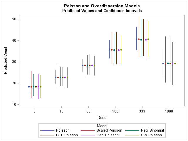
To visually show the effect of accounting for the overdispersion, these statements combine the predicted values and confidence intervals from the models and provide a comparative plot.
      data comp;
        set PredPoi (in=inp) PredPoiP (in=inpp) PredNB (in=innb)
            PredGEE (in=ingee) PredGP (in=ingp) PredCMP;
        length Model $14;
        if inp        then Model="Poisson";
        else if inpp  then Model="Scaled Poisson";
        else if innb  then Model="Neg. Binomial";
        else if ingee then Model="GEE Poisson";
        else if ingp  then Model="Gen. Poisson";
        else               Model="C-M Poisson";
        run;

      proc sgplot;
        highlow x=dose high=upper low=lower / group=Model
                groupdisplay=cluster clusterwidth=.5;
        scatter x=dose y=pred / group=Model
                groupdisplay=cluster clusterwidth=.5
                markerattrs=(symbol=circlefilled size=6);
        xaxis type=discrete label="Dose";
        yaxis label="Predicted Count";
        title "Poisson and Overdispersion Models";
        title2 "Predicted Values and Confidence Intervals";
        run;
Notice that accounting for the overdispersion with the various models above increases the variability around the predicted values relative to the Poisson model though the point estimates are very similar.
 |
Overdispersion resulting from zero inflation
Another possible cause of overdispersion is zero inflation. This example from Long (1997) uses data on the number of scientific articles published by doctoral candidates appearing in the PROC COUNTREG documentation in the SAS/ETS® User's Guide. The following statements fit a Poisson model to the number of articles, ART, using binary indicator variables indicating female gender, FEM, and married status, MAR.
These statements add a variable that indicates if the response, ART, equals zero and then computes the mean and variance of ART and the proportion of zeros in each FEM-MAR population. The final DATA step adds the proportion of zeros expected in each population under the Poisson distribution given its mean.
      data a;
        set long97data;
        zero=(art=0);
        run;
      proc means data=a mean var nway;
        class fem mar; var art zero;
        output out=mns mean=mu ObsProb0 var(art)=variance;
        run;
      data mns;
        set mns;
        PoiProb0=pdf("poisson",0,mu);
        run;
      proc print data=mns;
        id fem mar;
        var mu variance ObsProb0 PoiProb0;
        run;
Note that the variance in each population exceeds the mean estimate, mu, suggesting overdispersion. Also, the observed proportion of zeros (ObsProb0) exceeds the expected proportion (PoiProb0) under the Poisson distribution suggesting that this is the cause of the overdispersion.
|
The following statements fit a Poisson model to the data and saves the predicted values and confidence limits in data set PredPoi.
      proc genmod data=a;
         model art=fem mar / dist=p;
         output out=PredPoi p=predicted l=lclm u=uclm;
         run;
The Pearson/DF and Deviance/DF statistics are both close to 2 which provides some indication of overdispersion.
|
||||||||||||||||||||||||||||||||||||||||||||||||||||||||||||||||||||||||||||||||||||||||||||
Assuming that the extra zeros appearing in the data are causing overdispersion, a zero-inflated Poisson (ZIP) model can be fit. The ZIP (and related zero-inflated negative binomial (ZINB) model) is a two-part model with one model for the process that generates counts under the ordinary Poisson distribution and another (typically logistic) model for the process that generates extra zeros The MODEL statement specifies the first model and the ZEROMODEL statement specifies the model for the zero inflation parameter in the extra zeros process. For more details on this model, see "Zero-Inflated Models" in the Details section of the GENMOD documentation.
In the statements that follow, the Poisson counts are modeled using FEM and MAR as predictors. The ZEROMODEL statement specifies an intercept-only model for the probability of extra zeros. Any variables in the input data can be used as predictors in the zero inflation model, if desired, and can be different from those used in the MODEL statement. The fitted model is saved by the STORE statement and then reused in PROC PLM to estimate and save the predicted values and confidence limits under the ZIP model.
      proc genmod data=a;
        model art=fem mar / dist=zip;
        zeromodel;
        store zip;
        run;
      proc plm restore=zip;
        score data=a out=PredZIP pred stderr lclm uclm / ilink;
        run;
The parameter estimates under the ZIP model have increased slightly in response to the overdispersion from extra zeros. The intercept in the zero inflation model, -1.3792, is significant (p<0.0001). The AIC is smaller for the ZIP model than for the ordinary Poisson model suggesting it is the better model.
|
||||||||||||||||||||||||||||||||||||||||||||||||||||||||||||||||||||||||||||||||||||||||||||||||||||||||||||||||||||
The following combines the estimates and confidence limits from the Poisson and ZIP models and produces a comparative plot.
data comp;
set PredPoi (in=inp) PredZIP;
length Model $14;
if inp then Model="Poisson";
else Model="Z.I. Poisson";
FemMar=cats(fem,mar);
run;
proc sgplot;
highlow x=FemMar high=uclm low=lclm / group=Model
groupdisplay=cluster clusterwidth=.2;
scatter x=FemMar y=predicted / group=Model
groupdisplay=cluster clusterwidth=.2 markerattrs=(symbol=circlefilled size=6);
xaxis type=discrete label="Female/Married";
yaxis label="Predicted Count";
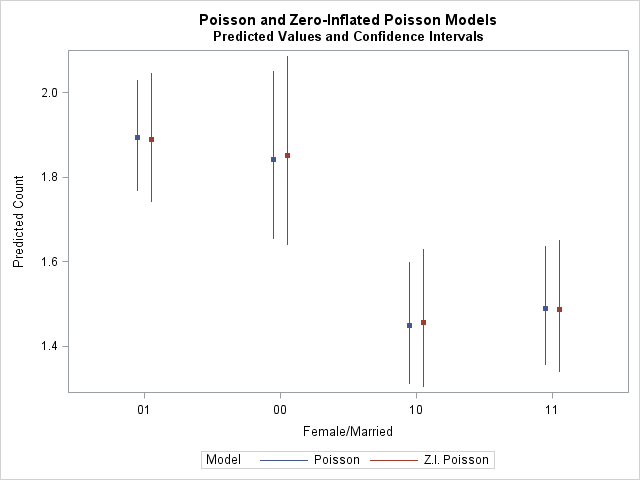
title "Poisson and Zero-Inflated Poisson Models";
title2 "Predicted Values and Confidence Intervals";
run;
The confidence intervals are a bit wider under the ZIP model adjusting for the overdispersion caused by extra zeros.
 |
Underdispersion
When the variance in the data is less than the Poisson mean, μ, the data are underdispersed. These statements create a variation on the assay data above to be used in the underdispersion models that follow.
      data assay;
        input dose salm @@;
        l_dose10 = log(dose+10);
        plate = _n_;
        datalines;
      0    15    0 16    0 18
      10   16   10 18   10 21
      33   20   33 22   33 19
      100  35  100 39  100 37
      333  33  333 38  333 37
      1000 20 1000 22 1000 25
      ;
As before, these statements estimate the mean and variance in each Dose population.
     proc means data=assay mean var;
       class dose;
       var salm;
       run;
In each Dose population, the variance is noticeably less than the mean suggesting underdispersion.
|
||||||||||||||||||||||||||||||||
Poisson model
The following statements fit the same ordinary Poisson model as above to these new data.
      proc genmod data=assay;
        model salm = dose l_dose10 / dist=poisson;
        output out=PredPoi p=pred l=lower u=upper;
        run;
The ordinary Poisson model shows some evidence of underdispersion since the Pearson/DF and Deviance/DF values are substantially less than 1.
|
||||||||||||||||||||||||||||||||||||||||||||||||||||||||||||||||||||||||||||||||||||||||||||
Scaled Poisson model
These statements add a scale parameter to the Poisson distribution which is estimated using the Pearson statistic.
      proc genmod data=assay;
        model salm = dose l_dose10 / dist=poisson scale=pearson;
        output out=PredSP p=pred l=lower u=upper;
        run;
Note that the Pearson/DF and Deviance/DF statistics are now equal to or close to 1. Also notice that the standard errors are now reduced from the ordinary Poisson model where the underdispersion inflated them.
|
||||||||||||||||||||||||||||||||||||||||||||||||||||||||||||||||||||||||||||||||||||||||||||
Generalized Estimating Equations model
The following fits a Poisson GEE model to correct for the underdispersion.
      proc genmod data=assay;
        class plate;
        model salm = dose l_dose10 / dist=poisson;
        repeated subject=plate;
        output out=PredGEE p=pred l=lower u=upper;
        run;
The effect of the GEE method on the parameter standard errors is somewhat greater than the Pearson scaling above. The standard errors are a bit smaller.
|
||||||||||||||||||||||||||||||||||||||||||
Generalized Poisson model
The GP model can also be used in cases of underdispersion and is fit by the statements below. PROC FMM cannot be used in the case of underdispersion because that procedure restricts its scale parameter to be positive.
      proc nlmixed data=assay;
        parms b0=2 b1=0 b2=0 xi=.1;
        y=salm;
        lp=b0 + b1*dose + b2*l_dose10;
        mu=exp(lp);
        mustar = mu - xi*(mu - y);
        ll = log(mu*(1-xi)) + (y-1)*log(mustar) - mustar - lgamma(y+1);
        model y ~ general(ll);
        predict mu out=PredGP;
        run;
The estimate of ξ is -0.5935 indicating significant underdispersion (p=0.0389). The adjustment for underdispersion falls somewhere between the scaled Poisson and the GEE models with the sizes of the parameter standard errors in between those two models. The smaller AIC suggests the GP model is better than the Poisson model.
|
||||||||||||||||||||||||||||||||||||||||||||||||||||||||||||||||
Conway-Maxwell Poisson model
These statements fit the CMP model and save the predicted valuesnote and estimates of the μ and ν distribution parameters. The NLEST macro is then used to obtain confidence intervals for the predicted means.
     proc countreg data=assay;
        model salm = dose l_dose10 / dist=cmp covb;
        output out=CMPpreds pred=pred mu=mu nu=nu;
        ods output parameterestimates=pe covb=c;
        run;
     %nlest(inest=pe, incovb=c,
        f=(exp(B_p1+B_p2*dose+B_p3*l_dose10))+1/(2*exp(-B_p4))-0.5,
        score=assay, outscore=PredCMP)
In the results, the negative value for -ln(ν), -0.9192, is significant (p=0.0061) and is evidence of underdispersion. The values for μ and ν in the CMPpreds data set again seem to satisfy the rule of thumb for validity of using the NLEST macro discussed above.
|
||||||||||||||||||||||||||||||||||||||||||||||||||||||||||||
Comparison of underdispersion models
The following summarizes the fit criteria for the underdispersion, except for the GEE model which is not likelihood-based. The smallest values are seen for the generalized Poisson model, though the CMP model has very similar values.
|
These statements combine the predicted values and confidence intervals from the underdispersion models and provide a comparative plot.
data comp;
set PredPoi (in=inp) PredSP (in=insp) PredGEE(in=ingee) PredGP (in=ingp) PredCMP;
length Model $14;
if inp then Model="Poisson";
else if insp then Model="Scaled Poisson";
else if ingee then Model="GEE Poisson";
else if ingp then Model="Gen. Poisson";
else Model="C-M Poisson";
run;
proc sgplot;
highlow x=dose high=upper low=lower / group=Model
groupdisplay=cluster clusterwidth=.4;
scatter x=dose y=pred / group=Model
groupdisplay=cluster clusterwidth=.4
markerattrs=(symbol=circlefilled size=6);
xaxis type=discrete label="Dose";
yaxis label="Predicted Count";
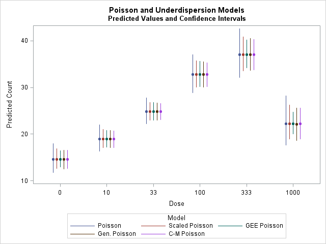
title "Poisson and Underdispersion Models";
title2 "Predicted Values and Confidence Intervals";
run;
All of the models for underdispersion show similar intervals that are narrower than the Poisson model. Again, the point estimates are very similar.
 |
Underdispersion resulting from zero truncation
Another possible cause of underdispersion is zero truncation. In the following data, further discussed in this note, Y is the number of times each individual skunk was captured over several trappings. Individual skunks never trapped could not be recorded, so only counts of one or more appear in the data. The absence of zero counts makes these data an example of zero truncation. For data like this, the truncated Poisson (TP) distribution can be used.
     data skunk;
         input y freq year sex $ @@;
         datalines;
         1  1 77  F    2  2  77  F    3  4  77  F   4  2  77  F   5  1  77  F
         1  3 77  M    2  0  77  M    3  3  77  M   4  3  77  M   5  2  77  M  6  2 77  M
         1  7 78  F    2  7  78  F    3  3  78  F   4  1  78  F   5  2  78  F
         1  4 78  M    2  3  78  M    3  1  78  M
         ;
The following statements estimate the mean and variance in each population, defined as a combination of Sex and Year values.
     proc means data=skunk mean var;
       freq freq;
       class sex year;
       var y;
       run;
In each population, the variance is noticeably less than the mean suggesting underdispersion.
|
||||||||||||||||||||||||||||||
Fitting a Poisson model to the data shows some evidence of underdispersion with the Pearson/DF and Deviance/DF statistics well below 1. Predicted values and confidence limits are saved in data set PredPoi.
      proc genmod data=skunk;
         class sex year;
         freq freq;
         model y = sex|year / dist=poisson;
         output out=PredPoi p=pred l=lower u=upper;
         run;
|
||||||||||||||||||||||||||||||||||||||||||||||||||||||||||||||||||||||||||||||||||||||||||||||||||||||||||||||||||||||||||||||||||||||||||||||||||||||||||||||||||||
These statements fit the TP model using PROC FMM. Predicted values are saved in data set PredFMM. Note that PROC FMM can also fit the truncated negative binomial model with the DIST=TRUNCNEGBIN option. The truncated negative binomial model is discussed and illustrated in this note.
      proc fmm data=skunk;
         class sex year;
         freq freq;
         model y = sex|year / dist=truncpoisson;
         output out=PredFMM pred;
         run;
Note that the parameter estimates from the TP model deviate farther from zero and have larger standard errors than under the ordinary Poisson model. The smaller AIC indicates a better fit from the truncated model.
|
|||||||||||||||||||||||||||||||||||||||||||||||||||||||||||||||||||||||||||||||||||||||||
Since the OUTPUT statement in PROC FMM does not offer confidence limits for the predicted values, the TP model can also be fitted in PROC NLMIXED by specifying its log likelihood function. The expression for the mean of the TP distribution is specified in the PREDICT statement which then saves the predicted values and confidence limits in data set PredTP. The results match those from PROC FMM above. PROC NLMIXED can also fit the truncated negative binomial model as shown in this note
      proc nlmixed data=skunk;
         parms b0=0 bf=0 b77=0 bf77=0;
         lambda=exp(b0 + bf*(sex="F") + b77*(year=77) + bf77*(sex="F")*(year=77));
         LL=freq*(-lambda+y*log(lambda)-lgamma(y+1)-log(1-exp(-lambda)));
         model y ~ general(LL);
         predict lambda/(1-exp(-lambda)) out=PredTP;
         run;
The following statements combine the predicted values and confidence intervals from the Poisson and TP models and provide a comparative plot.
data comp;
set PredPoi (in=inp) PredTP;
length Model $14;
if inp then Model="Poisson";
else Model="Trunc. Poisson";
SexYear=cats(sex,year);
run;
proc sgplot;
highlow x=SexYear high=upper low=lower / group=Model
groupdisplay=cluster clusterwidth=.2;
scatter x=SexYear y=pred / group=Model
groupdisplay=cluster clusterwidth=.2 markerattrs=(symbol=circlefilled size=6);
xaxis type=discrete label="Sex and Year";
yaxis label="Predicted Count";
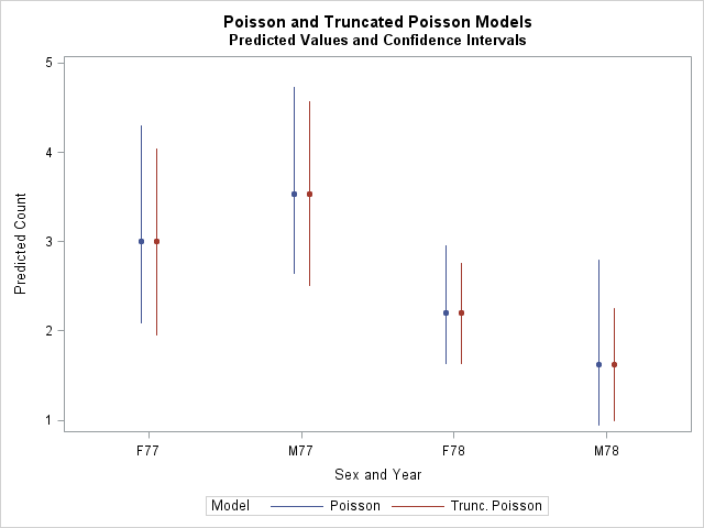
title "Poisson and Truncated Poisson Models";
title2 "Predicted Values and Confidence Intervals";
run;
Notice the narrower confidence intervals particularly at Year=78. The slight shift in the intervals occurs because of the different ways that GENMOD and NLMIXED estimate the interval limits. The intervals produced by GENMOD are not necessarily symmetrical about the mean estimates, while those from NLMIXED are.
 |
__________
Note: The predicted values provided by the PRED= option in the OUTPUT statement in PROC COUNTREG might differ from those computed by the NLEST macro. The macro always evaluates the expression that approximates the mean as specified in the f= option of the macro. However, the PRED= option in COUNTREG avoids using this approximation when μ<20 which suggests that the approximation might be less precise. A more precise computation is then done by the procedure. However, in cases where the above rule of thumb is slightly violated, the values from the macro and the procedure typically do not differ greatly.
Operating System and Release Information
| Product Family | Product | System | SAS Release | |
| Reported | Fixed* | |||
| SAS System | SAS/STAT | z/OS | ||
| Z64 | ||||
| OpenVMS VAX | ||||
| Microsoft® Windows® for 64-Bit Itanium-based Systems | ||||
| Microsoft Windows Server 2003 Datacenter 64-bit Edition | ||||
| Microsoft Windows Server 2003 Enterprise 64-bit Edition | ||||
| Microsoft Windows XP 64-bit Edition | ||||
| Microsoft® Windows® for x64 | ||||
| OS/2 | ||||
| Microsoft Windows 8 Enterprise 32-bit | ||||
| Microsoft Windows 8 Enterprise x64 | ||||
| Microsoft Windows 8 Pro 32-bit | ||||
| Microsoft Windows 8 Pro x64 | ||||
| Microsoft Windows 8.1 Enterprise 32-bit | ||||
| Microsoft Windows 8.1 Enterprise x64 | ||||
| Microsoft Windows 8.1 Pro | ||||
| Microsoft Windows 8.1 Pro 32-bit | ||||
| Microsoft Windows 95/98 | ||||
| Microsoft Windows 2000 Advanced Server | ||||
| Microsoft Windows 2000 Datacenter Server | ||||
| Microsoft Windows 2000 Server | ||||
| Microsoft Windows 2000 Professional | ||||
| Microsoft Windows NT Workstation | ||||
| Microsoft Windows Server 2003 Datacenter Edition | ||||
| Microsoft Windows Server 2003 Enterprise Edition | ||||
| Microsoft Windows Server 2003 Standard Edition | ||||
| Microsoft Windows Server 2003 for x64 | ||||
| Microsoft Windows Server 2008 | ||||
| Microsoft Windows Server 2008 R2 | ||||
| Microsoft Windows Server 2008 for x64 | ||||
| Microsoft Windows Server 2012 Datacenter | ||||
| Microsoft Windows Server 2012 R2 Datacenter | ||||
| Microsoft Windows Server 2012 R2 Std | ||||
| Microsoft Windows Server 2012 Std | ||||
| Microsoft Windows XP Professional | ||||
| Windows 7 Enterprise 32 bit | ||||
| Windows 7 Enterprise x64 | ||||
| Windows 7 Home Premium 32 bit | ||||
| Windows 7 Home Premium x64 | ||||
| Windows 7 Professional 32 bit | ||||
| Windows 7 Professional x64 | ||||
| Windows 7 Ultimate 32 bit | ||||
| Windows 7 Ultimate x64 | ||||
| Windows Millennium Edition (Me) | ||||
| Windows Vista | ||||
| Windows Vista for x64 | ||||
| 64-bit Enabled AIX | ||||
| 64-bit Enabled HP-UX | ||||
| 64-bit Enabled Solaris | ||||
| ABI+ for Intel Architecture | ||||
| AIX | ||||
| HP-UX | ||||
| HP-UX IPF | ||||
| IRIX | ||||
| Linux | ||||
| Linux for x64 | ||||
| Linux on Itanium | ||||
| OpenVMS Alpha | ||||
| OpenVMS on HP Integrity | ||||
| Solaris | ||||
| Solaris for x64 | ||||
| Tru64 UNIX | ||||
| Type: | Usage Note |
| Priority: | |
| Topic: | Analytics ==> Categorical Data Analysis Analytics ==> Regression SAS Reference ==> Procedures ==> NLMIXED SAS Reference ==> Procedures ==> FMM SAS Reference ==> Procedures ==> GENMOD SAS Reference ==> Procedures ==> HPFMM SAS Reference ==> Procedures ==> COUNTREG SAS Reference ==> Procedures ==> HPCOUNTREG |
| Date Modified: | 2020-09-11 12:05:13 |
| Date Created: | 2015-09-04 15:01:50 |