Usage Note 52161: Fitting the zero-inflated binomial model to overdispersed binomial data
 |  |  |
As with count models, such as Poisson and negative binomial models, overdispersion can also be seen in binomial models, such as logistic and probit models, meaning that the amount of variability in the data exceeds that of the binomial distribution. One possible cause of overdispersion is an excess of zero values. In such cases, a zero-inflated binomial (ZIB) model can be fit using PROC FMM. The following example illustrates fitting the ZIB model, testing its fit, and comparing it to the fit of a binomial (logistic) model.
For additional discussion of overdispersion see this note.
Example
The following data set appears in Friendly (2000) and is used in this note to test the fit of a Poisson model. The data are counts of the number of event occurrences in each of 262 sets of 200 trials. In this example, binomial and zero-inflated binomial models are fit to the data and the fit of the models is tested and compared.
These statements create the data set and fit a logistic model. Since there is only one population, there is a single predicted probability from the binomial model and this value appears in the Binp variable in the data set created by the OUTPUT statement.
      data Madison;
         input y freq;
         n=200;
         Observed=freq/262;
         datalines;
         0  156
         1   63
         2   29
         3    8
         4    4
         5    1
         6    1
         ;
      proc logistic data=Madison;
         freq freq;
         model y/n = ;
         output out=bin p=Binp;
         run;
The following statements compute the estimated probabilities Pr(Y=0), Pr(Y=1), ... , Pr(Y=6) under the fitted binomial model, saves them in the PredBin variable in the BINEXP data set, and displays them.
      data binexp;
         set bin;
         PredBin=pdf("binomial",y,binp,262);
         label PredBin="Binomial Prob";
         run;
      proc print label;
         id y;
         var Observed PredBin;
         run;
|
The small expected probabilities beyond Y=3 could cause unreliability of the Pearson chi-square statistic, so these statements combine those probabilities in the variable _TESTP_.
      proc format;
         value yfmt 3-high = "3+";
         run;
      proc means data=binexp sum nway;
         by y;
         var Observed PredBin;
         format y yfmt.;
         output out=binexpagg sum=Observed _testp_;
         run;
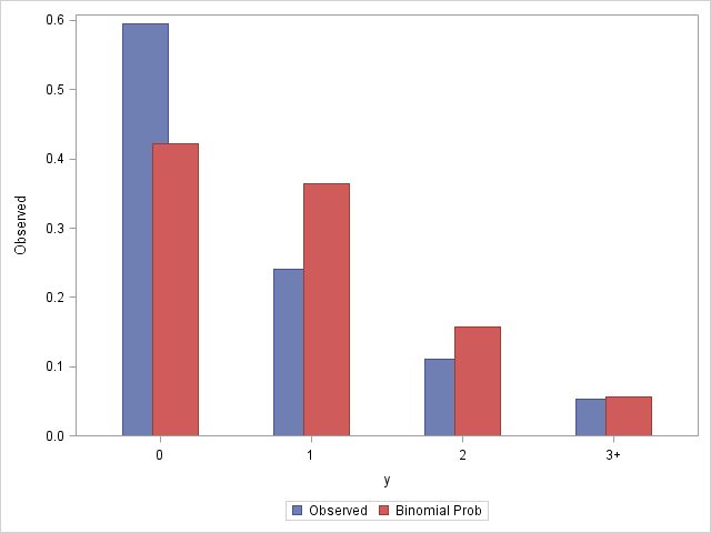
These statements produce a bar chart showing how the binomial model deviates from the observed probabilities.
      proc sgplot;
         vbarparm category=y response=Observed / discreteoffset=-.1 barwidth=.3;
         vbarparm category=y response=_testp_  / discreteoffset=.1 barwidth=.3;
         run;
Notice that the observed data shows an excess of zero values compared to the binomial model.

|
A test of the fit of the binomial model can now be done using the CHISQ option in PROC FREQ. The TESTP= option uses the _TESTP_ variable in the specified data set (BINEXPAGG) to supply the expected probabilities for the Pearson chi-square test. Since the intercept in the logistic model estimates the binomial mean (Binp), one additional degree of freedom must be subtracted and this is done with the DF=-1 option.
      proc freq data=Madison;
         weight freq;
         table y / chisq(testp=binexpagg df=-1);
         ods select OneWayChiSq;
         format y yfmt.;
         run;
The significant result (p< 0.0001) indicates that the Binomial model does not fit well.
| ||||||||
To accommodate the excess zeros, a zero-inflated binomial (ZIB) model can be fit using PROC FMM. Zero-inflation can be added to any model using a second MODEL statement and the CONSTANT distribution as shown in the following statements. The OUTPUT statement saves the overall predicted value (PRED) and the mixing probabilities for the two components of the mixture model — the logistic component (MP_1) and the zero-inflation component (MP_2).
      proc fmm data=Madison;
         freq freq;
         model y/n =  / dist=binomial;
         model  +     / dist=constant;
         output out=zib pred=pred mixprobs=mp;
         run;
As was done for the Binomial model, the probabilities for each level of Y are computed and the small probabilities at Y=3 and beyond are aggregated.
      data zibexp;
         set zib;
         munozero = pred/mp_1;
         comb = lgamma(n+1) - lgamma(y+1) - lgamma(n-y+1);
         PredZIB = exp(log(mp_1) + comb + y*log(munozero) +
                   (n-y)*log(1-munozero)) + (1-mp_1)*(y=0);
         label PredZIB="ZI Binomial Prob";
         run;
      proc means data=zibexp sum nway;
         by y;
         var Observed PredZIB;
         format y yfmt.;
         output out=zibexpagg sum=Observed _testp_;
         run;
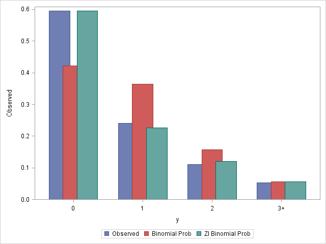
These statements display the observed probabilities along with the predicted probabilities for the response levels under the binomial and ZIB models.
      data preds;
         merge binexpagg(rename=(_testp_=PredBin))
               zibexpagg(rename=(_testp_=PredZIB));
         run;
      proc print label;
         id y;
         var Observed PredBin PredZIB;
         run;
      proc sgplot;
         vbarparm category=y response=Observed / discreteoffset=-.2 barwidth=.3;
         vbarparm category=y response=PredBin  / discreteoffset=0 barwidth=.3;
         vbarparm category=y response=PredZIB  / discreteoffset=.2 barwidth=.3;
         run;
Notice that the ZIB model does a much better job of handling the probability of Y=0 and generally follows the observed distribution much better than the binomial model.

|
The Pearson goodness of fit test can again be used to assess the model fit. The ZIB model requires estimation of both an intercept in the logistic component of the model and a mixing probability (the other mixing probability is constrained so that their sum is one). Since two parameters are estimated, the DF=-2 option is used to decrease the degrees of freedom of the Pearson statistic by 2.
      proc freq data=Madison;
         weight freq;
         table y / chisq(testp=zibexpagg df=-2);
         ods select OneWayChiSq;
         format y yfmt.;
         run;
The insignificant result (p=0.4865) confirms the visual impression that the ZIB model is a good fit to the observed data.
| ||||||||
________
Friendly, M. (2000), Visualizing Categorical Data, Cary, NC: SAS Institute Inc.
Operating System and Release Information
| Product Family | Product | System | SAS Release | |
| Reported | Fixed* | |||
| SAS System | SAS/STAT | z/OS | ||
| Z64 | ||||
| OpenVMS VAX | ||||
| Microsoft® Windows® for 64-Bit Itanium-based Systems | ||||
| Microsoft Windows Server 2003 Datacenter 64-bit Edition | ||||
| Microsoft Windows Server 2003 Enterprise 64-bit Edition | ||||
| Microsoft Windows XP 64-bit Edition | ||||
| Microsoft® Windows® for x64 | ||||
| OS/2 | ||||
| Microsoft Windows 8 Enterprise 32-bit | ||||
| Microsoft Windows 8 Enterprise x64 | ||||
| Microsoft Windows 8 Pro 32-bit | ||||
| Microsoft Windows 8 Pro x64 | ||||
| Microsoft Windows 8.1 Enterprise 32-bit | ||||
| Microsoft Windows 8.1 Enterprise x64 | ||||
| Microsoft Windows 8.1 Pro | ||||
| Microsoft Windows 8.1 Pro 32-bit | ||||
| Microsoft Windows 95/98 | ||||
| Microsoft Windows 2000 Advanced Server | ||||
| Microsoft Windows 2000 Datacenter Server | ||||
| Microsoft Windows 2000 Server | ||||
| Microsoft Windows 2000 Professional | ||||
| Microsoft Windows NT Workstation | ||||
| Microsoft Windows Server 2003 Datacenter Edition | ||||
| Microsoft Windows Server 2003 Enterprise Edition | ||||
| Microsoft Windows Server 2003 Standard Edition | ||||
| Microsoft Windows Server 2003 for x64 | ||||
| Microsoft Windows Server 2008 | ||||
| Microsoft Windows Server 2008 R2 | ||||
| Microsoft Windows Server 2008 for x64 | ||||
| Microsoft Windows Server 2012 Datacenter | ||||
| Microsoft Windows Server 2012 R2 Datacenter | ||||
| Microsoft Windows Server 2012 R2 Std | ||||
| Microsoft Windows Server 2012 Std | ||||
| Microsoft Windows XP Professional | ||||
| Windows 7 Enterprise 32 bit | ||||
| Windows 7 Enterprise x64 | ||||
| Windows 7 Home Premium 32 bit | ||||
| Windows 7 Home Premium x64 | ||||
| Windows 7 Professional 32 bit | ||||
| Windows 7 Professional x64 | ||||
| Windows 7 Ultimate 32 bit | ||||
| Windows 7 Ultimate x64 | ||||
| Windows Millennium Edition (Me) | ||||
| Windows Vista | ||||
| Windows Vista for x64 | ||||
| 64-bit Enabled AIX | ||||
| 64-bit Enabled HP-UX | ||||
| 64-bit Enabled Solaris | ||||
| ABI+ for Intel Architecture | ||||
| AIX | ||||
| HP-UX | ||||
| HP-UX IPF | ||||
| IRIX | ||||
| Linux | ||||
| Linux for x64 | ||||
| Linux on Itanium | ||||
| OpenVMS Alpha | ||||
| OpenVMS on HP Integrity | ||||
| Solaris | ||||
| Solaris for x64 | ||||
| Tru64 UNIX | ||||
| Type: | Usage Note |
| Priority: | |
| Topic: | SAS Reference ==> Procedures ==> FMM Analytics ==> Categorical Data Analysis Analytics ==> Distribution Analysis Analytics ==> Regression |
| Date Modified: | 2014-02-07 15:56:44 |
| Date Created: | 2014-01-22 16:59:44 |