Usage Note 46997: Estimating the risk (proportion) difference for matched pairs data with binary response
 |  |  |
For matched pairs data with a binary response (such as yes/no responses from husband and wife pairs), the AGREE option in PROC FREQ provides a test of equal probability of a Yes response. This is McNemar's test of marginal homogeneity. Point and confidence interval estimates of the risk difference for paired data can be obtained using either a stratification method with the COMMONRISKDIFF option in PROC FREQ or using a model-based approach. Model-based methods use either a linear probability model that estimates the event probabilities directly or a Generalized Estimating Equations (GEE) model. With a GEE model, the risk difference can be estimated using the Margins macro to compute predictive margins and their difference or using the NLMeans macro to estimate the appropriate nonlinear functions of the model parameters. These methods are discussed and illustrated below.
To estimate the risk difference between independent groups, rather than in matched pairs, see SAS Note 37228. For estimating the odds ratio with matched pairs data, see SAS Note 23127.
Paired Data Example
In this example, 100 husband and wife pairs were asked a question that could be answered Yes or No. The results are recorded in the following data set. The Yes response is coded 1 and No is coded 0. Since only four distinct response combinations are possible, the data can be summarized as the number of pairs (Npairs) with each possible combination:
     data hwpairs;
       input husband wife Npairs;
       datalines;
       1 1 15
       1 0 20
       0 1 5
       0 0 60
       ;
Test of Marginal Homogeneity in PROC FREQ
To test that the proportion of husbands answering Yes is equal to the number of wives answering Yes, McNemar's test of marginal homogeneity (equal marginal probabilities) can be obtained using the AGREE option in PROC FREQ:
     proc freq data=hwpairs;
       table husband*wife / agree;
       weight Npairs;
       run;
The results show that the husband and wife probabilities differ significantly (p=0.0027). The marginal percentages for the HUSBAND=1 row and the WIFE=1 column show that 35% of husbands and 20% of wives answered Yes – a difference of 15%:
|
||||||||||||||||||||||||||||||||||||||||||||||||||||||||||||||||||||
Stratified Analysis in PROC FREQ
In order to estimate the risk difference, its standard error, and confidence interval, the data needs to be rearranged as a stratified table. The model-based methods require the same data arrangement in which observations contain individual responses rather than summarized data as above. The following DATA step expands the summarized data above into a data set containing an observation for each member (husband or wife) of each pair. A variable identifying the pair (ID) is created. The DO loop splits each observation of the summary data into two observations for each pair in each response combination resulting in 200 observations. Husband or wife is indicated by the MEMBER variable (1=husband, 2=wife), and the responses from all subjects are stored in the RESPONSE variable:
     data indiv;
       set hwpairs;
       retain id 0;
       do id=id+1 to id+Npairs;
         member=1; response=husband; output;
         member=2; response=wife; output;
       end;
       keep id member response;
       run;
These statements display the observations for the first four pairs, which were all from the yes/yes response combination:
     proc print data=indiv (obs=8);
       id id;
       run;
|
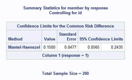
These statements create the stratified table (member by response stratified by pair) and use the COMMONRISKDIFF option to estimate the common risk difference computed across the strata (ID). By default or with the CL=MH suboption, PROC FREQ uses the Mantel-Haenszel type of confidence limits, but several other types are available. See the description of the COMMONRISKDIFF option in the PROC FREQ documentation. The NOPRINT option avoids printing the table for each stratum:
     proc freq data=indiv order=data;
       table id*member*response / commonriskdiff(cl=mh) noprint;
       run;
As seen from the table of summarized observed data above, the estimated risk difference is 0.15 with a 95% confidence interval of (0.0565, 0.2435):
 |
GEE Analysis
PROC GEE or PROC GENMOD can be used to fit a repeated measures logistic model to the individual level data. The NLMeans macro (SAS Note 62362) can then be used to estimate the difference of the Yes probabilities.
In the following statements, the EVENT='1' response variable option tells GENMOD to model the probability of a RESPONSE=1 (Yes). Since husband and wife responses are considered correlated, the pair identifier (ID) is used in the SUBJECT= option in the REPEATED statement. The LSMEANS statement with the ILINK and CL options estimates the Yes probabilities for husbands and wives and provides confidence intervals. The E option produces a table of the coefficients defining the LSMEANS. This table is saved by the ODS OUTPUT statement. The STORE statement saves the fitted model. The coefficients table and the stored model are used by the NLMeans macro:
     proc genmod data=indiv;
       class id member;
       model response(event='1') = member / dist=binomial;
       repeated subject=id;
       lsmeans member / ilink cl e;
       ods output coef=c;
       store geemod;
       run;
The husband and wife probability estimates are shown in the Mean column of the "member Least Squares Means" table. 95% confidence limits for each are also provided:
|
||||||||||||||||||||||||||||||||||||||||||||||||
Using the NLMeans Macro to Estimate the Risk Difference
See the description of the NLMeans macro (SAS Note 62362) for information about obtaining the latest release and making it available in your SAS®session.
The following call of the NLMeans macro also estimates the difference in the husband and wife probabilities. In addition to specifying the saved model and the table of LSMEANS coefficients, the link function used in the model is specified. A title for the table is also given:
%NLMeans(instore=geemod, coef=c, link=logit, title=Pr(Yes) Difference)
The results match those from the COMMONRISKDIFF option in PROC FREQ above. The difference in the probabilities, 0.15, is shown in the Estimate column of the table along with the standard error of the difference (0.0477) and a 95% confidence interval (0.0565, 0.2435). The test of the difference indicates that the husband and wife probabilities differ (p=0.0017). The Label indicates the direction of the difference in proportions is member1-member2 or husband-wife. If the reverse is desired, then specify options=reverse in the NLMeans macro call:
|
Using the Margins Macro to Estimate the Risk Difference
See the description of the Margins macro (SAS Note 63038) for information about obtaining the latest release and making it available in your SAS®session.
The Margins macro fits the specified model and computes estimates of the response mean for each level of the margins= variable. Each mean estimate is a predictive margin – an average of the predicted values when all observations are fixed at one a level of the margins= variable. For this example, the predictive margins for husbands and wives are estimates of the probability of a Yes response. The risk difference is considered the marginal effect of the MEMBER predictor.
In the following call of the Margins macro, the same logistic GEE model as above is requested by the class=, response=, roptions=, dist=, model=, and geesubject= specifications. The predictive margins for husbands and wives are requested by margins=member. An estimate and confidence interval of the husband-wife risk difference, the marginal effect, is provided by options=diff cl:
   %Margins(data       = indiv,
            class      = id member,
            response   = response,
            roptions   = event='1',
            dist       = binomial,
            model      = member,
            geesubject = id,
            margins    = member,
            options    = diff cl)
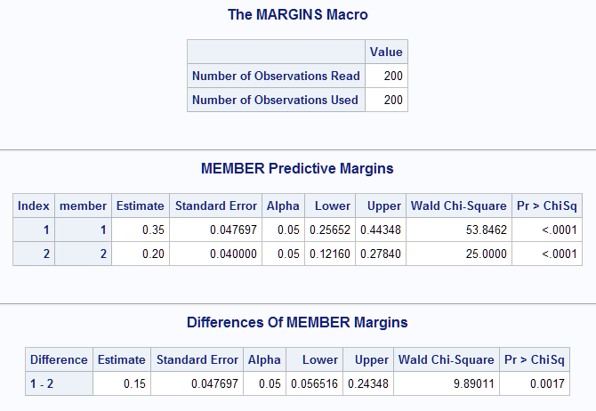
The estimated predictive margins for husbands and wives match the estimates from the LSMEANS statement in PROC GENMOD above. The MEMBER marginal effect, or difference in husband and wife means, is estimated to be 0.15 with a confidence interval (0.0565, 0.2435). The test of the difference indicates that husbands have significantly higher probability of responding Yes than wives (p=0.0017). The label in the Difference column indicates the direction of the difference is member1-member2 or husband-wife. If the reverse is desired, then specify reverse in options= in the Margins macro call:
 |
Using a Linear Probability Model and LSMEANS/DIFF
Alternatively, the difference in probabilities can be estimated by modeling the probability of a Yes response directly. The DIST=BINOMIAL and LINK=IDENTITY options fit a linear probability model.Note With the probability modeled directly, the LSMEANS estimates are the estimated probabilities and the DIFF option can be used to estimate the difference in probabilities:
     proc genmod data=indiv;
       class id member;
       model response(event='1') = member / dist=binomial link=identity;
       repeated subject=id;
       lsmeans member / diff cl;
       run;
The husband and wife probability estimates and difference again match the above results from the Margins and NLMeans macros:
|
|||||||||||||||||||||||||||||||||||||||||||||||||||||||||||
_____
Note: Unlike the default logit link function, the identity link does not ensure that the model produces valid probability estimates. Errors might result when fitting such models depending on the model and the data.
Operating System and Release Information
| Product Family | Product | System | SAS Release | |
| Reported | Fixed* | |||
| SAS System | SAS/STAT | z/OS | ||
| OpenVMS VAX | ||||
| Microsoft® Windows® for 64-Bit Itanium-based Systems | ||||
| Microsoft Windows Server 2003 Datacenter 64-bit Edition | ||||
| Microsoft Windows Server 2003 Enterprise 64-bit Edition | ||||
| Microsoft Windows XP 64-bit Edition | ||||
| Microsoft® Windows® for x64 | ||||
| OS/2 | ||||
| Microsoft Windows 8 | ||||
| Microsoft Windows 95/98 | ||||
| Microsoft Windows 2000 Advanced Server | ||||
| Microsoft Windows 2000 Datacenter Server | ||||
| Microsoft Windows 2000 Server | ||||
| Microsoft Windows 2000 Professional | ||||
| Microsoft Windows 2012 | ||||
| Microsoft Windows NT Workstation | ||||
| Microsoft Windows Server 2003 Datacenter Edition | ||||
| Microsoft Windows Server 2003 Enterprise Edition | ||||
| Microsoft Windows Server 2003 Standard Edition | ||||
| Microsoft Windows Server 2003 for x64 | ||||
| Microsoft Windows Server 2008 | ||||
| Microsoft Windows Server 2008 for x64 | ||||
| Microsoft Windows XP Professional | ||||
| Windows 7 Enterprise 32 bit | ||||
| Windows 7 Enterprise x64 | ||||
| Windows 7 Home Premium 32 bit | ||||
| Windows 7 Home Premium x64 | ||||
| Windows 7 Professional 32 bit | ||||
| Windows 7 Professional x64 | ||||
| Windows 7 Ultimate 32 bit | ||||
| Windows 7 Ultimate x64 | ||||
| Windows Millennium Edition (Me) | ||||
| Windows Vista | ||||
| Windows Vista for x64 | ||||
| 64-bit Enabled AIX | ||||
| 64-bit Enabled HP-UX | ||||
| 64-bit Enabled Solaris | ||||
| ABI+ for Intel Architecture | ||||
| AIX | ||||
| HP-UX | ||||
| HP-UX IPF | ||||
| IRIX | ||||
| Linux | ||||
| Linux for x64 | ||||
| Linux on Itanium | ||||
| OpenVMS Alpha | ||||
| OpenVMS on HP Integrity | ||||
| Solaris | ||||
| Solaris for x64 | ||||
| Tru64 UNIX | ||||
| Type: | Usage Note |
| Priority: | |
| Topic: | Analytics ==> Categorical Data Analysis Analytics ==> Longitudinal Analysis SAS Reference ==> Procedures ==> FREQ SAS Reference ==> Procedures ==> GENMOD SAS Reference ==> Macro |
| Date Modified: | 2024-01-11 16:15:38 |
| Date Created: | 2012-07-13 15:06:20 |