Sample 45576: Bayesian Hierarchical Poisson Regression Model for Overdispersed Count Data Using SAS/STAT 9.3
 |  |  |  |
Overview
This example uses the RANDOM statement in MCMC procedure to fit a Bayesian hierarchical Poisson regression model to overdispersed count data. The RANDOM statement, available in SAS/STAT 9.3 and later, provides a convenient way to specify random effects with substantionally improved performance. Overdispersion occurs when count data appear more dispersed than expected under a reference model. Overdispersion can be caused by positive correlation among the observations, an incorrect model, an incorrect distributional specification, or incorrect variance functions. The example displays how Bayesian hierarchical Poisson regression models are effective in capturing overdispersion and providing a better fit.
Analysis
Count data frequently display overdispersion (more variation than expected from a standard parametric model). Breslow (1984) discusses these types of models and suggests several different ways to model them. Hierarchical Poisson models have been found effective in capturing the overdispersion in data sets with extra Poisson variation.
Hierarchical Poisson regression models are expressed as Poisson models with a log link and a normal variance on the mean parameter. More formally, a hierarchical Poisson regression model is written as

|

|

|
|||

|

|

|
|||

|
|

|
for  ,
,  , and
, and  .
.
Consider data collected by Margolin, Kaplan, and Zeiger (1981) and studied in Breslow (1984) from an Ames salmonella mutagenicity assay. Table 1 reports the number of revertant colonies of TA98 salmonella (SALM) tested at six dose levels of quinoline (DOSE) with three replicate plates.
|
Doses of Quinoline ( |
|||||
|---|---|---|---|---|---|
|
0 |
10 |
33 |
100 |
333 |
1000 |
|
15 |
16 |
16 |
27 |
33 |
20 |
|
21 |
18 |
26 |
41 |
38 |
27 |
|
29 |
21 |
33 |
60 |
41 |
42 |
 g per plate)
The following statements read the data into SAS and create the ASSAY data set. The variable  models the mutagenic effect of quinoline. The value 10 is chosen because it is the smallest nonzero treatment level.
data assay;
   input dose salm @@;
   l_dose10 = log(dose+10);
   plate = _n_;
   datalines;
   0 15 0 21 0 29
   10 16 10 18 10 21
   33 16 33 26 33 33
   100 27 100 41 100 60
   333 33 333 38 333 41
   1000 20 1000 27 1000 42
   ;
The data appear to be a likely candidate for a Bayesian hierarchical Poisson regression model with replicates. However, you usually begin with a standard analysis of a Poisson regression and evaluate any evidence for overdispersion.
Bayesian Poisson Regression Model
Suppose you want to fit a Bayesian Poisson regression model for the frequency of revertant colonies of TA98 Salmonella with density

|
|

|
|||

|
|

|
(1) |
for the  plates, where
  represents the regression parameters and
  is the vector of covariates written as
  .
.
The likelihood function for each of the revertant colonies of salmonella and corresponding covariates is

|
(2) |
where  denotes
a conditional probability mass function. The Poisson density is evaluated at the specified value of
denotes
a conditional probability mass function. The Poisson density is evaluated at the specified value of  with a corresponding mean parameter
  . The three parameters,
  ,
,  , and
, and  , correspond to an intercept, the toxic effect for dose, and the mutagenic effect for dose, respectively.
Suppose the following prior distributions are placed on the parameters, where  indicates a prior distribution:

|
|

|
The diffuse  prior expresses your lack of knowledge about the regression parameters.
Using Bayes’ theorem, the likelihood function and prior distributions determine the posterior distribution of
 , and .
PROC MCMC obtains samples from the desired posterior distribution. You do not need to specify the exact form of the posterior distribution.
, and .
PROC MCMC obtains samples from the desired posterior distribution. You do not need to specify the exact form of the posterior distribution.
The goodness-of-fit Pearson chi-square statistic  as given in McCullagh and Nelder (1989) is calculated to assess model fit:

|
|

|
(3) |
First, let  and
and  represent an expectation and a variance, respectively, for a Poisson likelihood
  , where is defined in Equation 1.
If there is no overdispersion, the Pearson statistic approximately equals the number of observations in the data set minus the number of parameters in the model.
, where is defined in Equation 1.
If there is no overdispersion, the Pearson statistic approximately equals the number of observations in the data set minus the number of parameters in the model.
The following SAS statements use the likelihood function and diffuse prior distributions to fit the Bayesian Poisson regression model and calculate the Pearson chi-square statistic:
ods graphics on;
proc mcmc data=assay outpost=postout thin=5 seed=1181 nbi=10000 nmc=10000
   propcov=quanew monitor=(_parms_ Pearson) dic;
   parms beta1 2 beta2 0 beta3 0;
   prior beta: ~ normal(0,var=1000);
   lambda = exp(beta1 + beta2*dose + beta3*l_dose10);
   model salm ~ poisson(lambda);
   if plate eq 1 then Pearson = 0;
   Pearson =  Pearson + ((salm - lambda)**2/lambda);
run;
ods graphics off;
The PROC MCMC statement invokes the procedure and specifies the input data set. The OUTPOST= option specifies the output data set for posterior samples of parameters. The THIN= option controls the thinning of the Markov chain and specifies that one of every 5 samples is kept. Thinning is often used to reduce the correlations among posterior sample draws.The SEED= option specifies a seed for the random number generator (the seed guarantees the reproducibility of the random stream). The NBI= option specifies the number of burn-in iterations. The NMC= option specifies the number of posterior simulation iterations. The PROPCOV=QUANEW option uses the estimated inverse Hessian matrix as the initial proposal covariance matrix. The MONITOR=(_PARMS_ PEARSON) option outputs analysis on the _PARMS_ (which is shorthand for all model parameters) and the Pearson chi-square statistic. The DIC option specifies that the deviance information criterion (DIC) is requested.
The PARMS statement specifies the parameters in the model and assigns initial values to each of them. The PRIOR statements specify priors for all the parameters. The notation
beta: in the PRIOR statement is shorthand for all variables that start with beta. The shorthand notation is not necessary,
but it keeps your code succinct. The LAMBDA assignment statement calculates
for each observation in the Poisson model, as given in Equation 1. The MODEL statement specifies the Poisson function for SALM.
The next two lines of statements use SALM and LAMBDA (which are the expected value and the variance of the Poisson distribution, repectively) to calculate the Pearson chi-square statistic. The IF statement sets the value of PEARSON to 0 at the top of the data set (that is, when the value of the data set variable PLATE is 1). As PROC MCMC cycles through the data set at each iteration, the procedure cumulatively adds the Pearson chi-square statistic over each value of SALM. By the end of the data set, you obtain the Pearson chi-square statistic, as defined in Equation 3.
Figure 1 displays diagnostic plots to assess whether the Markov chains have converged.

The trace plot in Figure 1 indicates that the chain appears to have reached a stationary distribution. It also has good mixing and
is dense. The autocorrelation plot indicates low autocorrelation and efficient sampling. Finally, the kernel density plot shows close to a unimodal shape of posterior marginal
distribution for . The remaining
diagnostic plots (not shown here) similarly indicate good convergence in the other parameters.
PROC MCMC produces formal diagnostic tests by default. They are omitted here since informal checks on the chains, autocorrelation, and posterior density plots display stabilization and convergence.
Figure 2 reports summary and interval statistics for each parameter’s posterior distribution. PROC MCMC calculates the sampled value of the Pearson chi-square statistic at each iteration and produces its corresponding posterior summary statistics.
| Posterior Summaries | ||||||
|---|---|---|---|---|---|---|
| Parameter | N | Mean | Standard Deviation |
Percentiles | ||
| 25% | 50% | 75% | ||||
| beta1 | 2000 | 2.1768 | 0.2110 | 2.0391 | 2.1834 | 2.3142 |
| beta2 | 2000 | -0.00101 | 0.000233 | -0.00117 | -0.00101 | -0.00085 |
| beta3 | 2000 | 0.3184 | 0.0549 | 0.2817 | 0.3191 | 0.3549 |
| Pearson | 2000 | 49.3974 | 3.4673 | 46.8851 | 48.4551 | 50.7996 |
| Posterior Intervals | |||||
|---|---|---|---|---|---|
| Parameter | Alpha | Equal-Tail Interval | HPD Interval | ||
| beta1 | 0.050 | 1.7421 | 2.5790 | 1.7467 | 2.5798 |
| beta2 | 0.050 | -0.00148 | -0.00056 | -0.00146 | -0.00054 |
| beta3 | 0.050 | 0.2136 | 0.4288 | 0.2169 | 0.4305 |
| Pearson | 0.050 | 45.5715 | 59.2921 | 45.3427 | 56.2309 |
With  and three model parameters, the sampled value 49.4333 of the Pearson chi-square statistic is much greater than the desired
 ,
providing evidence of overdispersion. Although you have already captured the mutagenic and toxic effects, a Bayesian hierarchical Poisson model can also capture the observed excess
variation due to the replicate plates.
,
providing evidence of overdispersion. Although you have already captured the mutagenic and toxic effects, a Bayesian hierarchical Poisson model can also capture the observed excess
variation due to the replicate plates.
Figure 3 reports the calculated DIC (Spiegelhalter et al.; 2002) for the Bayesian Poisson regression model. The DIC is a model assessment tool and a Bayesian alternative to Akaike’s or Bayesian information criterion. The DIC can be applied to non-nested models and models that have data which are not independent an didentically distributed. When models with different DIC values are compared, a smaller DIC indicates a better fit to the data set. The DIC for this model is 141.882.
| Deviance Information Criterion | |
|---|---|
| Dbar (posterior mean of deviance) | 139.070 |
| Dmean (deviance evaluated at posterior mean) | 136.258 |
| pD (effective number of parameters) | 2.812 |
| DIC (smaller is better) | 141.882 |
Bayesian Hierarchical Poisson Regression Model
In overdispersed Poisson regression, the parameter estimates do not vary much from the Poisson model, but the estimated variance is inflated. Draper (1996) considers Bayesian hierarchical Poisson regression models for this type of data with density

|
|

|
|||
|
|
|

|
(4) | ||
|
|
|

|
for the
treatment levels and
replicates. The likelihood function is given in Equation 2, but now there are additional parameters in the model. You add random effects
 with a normal prior with mean
  and variance
  .
.
Suppose the priors are placed on the regression and variance parameters as follows:
|
|
|
|
|||

|
|

|
The mean and variance,  and
and  , respectively,
for the Pearson chi-square statistic in the hierarchical Poisson regression model are calculated using the iterated expectation and variance functions as
, respectively,
for the Pearson chi-square statistic in the hierarchical Poisson regression model are calculated using the iterated expectation and variance functions as

|
|
|
|||

|
|

|
(5) | ||
|
|
|

|
|||

|
|

|
|||
|
|
|

|
(6) |
The following SAS statements use the likelihood function and prior distributions to fit the Bayesian Poisson hierarchical regression model and calculate the Pearson chi-square statistic.
ods graphics on;
proc mcmc data=assay outpost=postout thin=5 seed=248601 nbi=10000 nmc=100000
   monitor=(beta1-beta3 Pearson) dic;

   parms beta1 2 beta2 0.01 beta3 0.5;
   parms s2 1;

   prior beta: ~ normal(0,var=1000);
   prior s2 ~ igamma(0.01, s=0.01);
   w = beta1 + beta2*dose + beta3*l_dose10;
   random gamma~ normal(0,var=s2) subject=plate;
   lambda = exp(w+gamma);
   model salm ~ poisson(lambda);

   mu = exp(w + s2/2);
   sigma2 = mu + (exp(s2) - 1)*(mu**2);
   if plate eq 1 then Pearson = 0;
   Pearson =  Pearson + ((salm - mu)**2/(sigma2));
run;
ods graphics off;
The first PARMS statement places all regression parameters in a single block and assigns them initial values. The second PARMS statement places the variance parameter in a separate block and assigns it an initial value of 1.
The PRIOR statement on the regression parameters does not change from the Poisson regression model.
The second PRIOR statement specifies the prior distribution for .
The W assignment statement calculates  for each observation.
The RANDOM statement specifies the random effect,  ,
with a normal prior distribution centered at with variance (s2).
The SUBJECT= option indicates the group index for the random effects parameters.
,
with a normal prior distribution centered at with variance (s2).
The SUBJECT= option indicates the group index for the random effects parameters.
The LAMBDA assignment statement calculates  , and the MODEL statement specifies the likelihood function for SALM as given in Equation 4.
The next four lines of statements use SALM and the sampled values of
and to calculate the Pearson chi-square statistic according to Equation 3. The moments are evaluated in the MU and SIGMA2 assignment variables according to Equation 5 and 6, respectively.
The diagnostic plot for is illustrated in Figure 4.
It displays the desired convergence, low autocorrelation, and smooth unimodal marginal posterior density for the parameter. The remaining diagnostic plots (not shown here) similarly indicate good convergence in the other parameters.
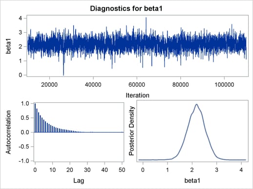
Figure 5 reports summary and interval statistics for the parameters and for the Pearson chi-square statistic. The fit statistic in the Bayesian hierarchical Poisson regression model is greatly reduced with a value of 19.4658, which suggests a much better fit compared to its value of 49.3974 in the Poisson regression model. The value of the fit statistic is now much closer to the desired number of observations minus the number of parameters.
Compared to the results in Figure 2, the parameter estimates for intercept and treatment change a small amount, their standard errors are inflated, and the confidence intervals are wider. Thus the treatment effect of quinoline does not decrease with the Bayesian hierarchical Poisson regression model.
| Posterior Summaries | ||||||
|---|---|---|---|---|---|---|
| Parameter | N | Mean | Standard Deviation |
Percentiles | ||
| 25% | 50% | 75% | ||||
| beta1 | 20000 | 2.1710 | 0.3635 | 1.9361 | 2.1770 | 2.4082 |
| beta2 | 20000 | -0.00097 | 0.000442 | -0.00125 | -0.00097 | -0.00069 |
| beta3 | 20000 | 0.3117 | 0.0994 | 0.2462 | 0.3105 | 0.3754 |
| Pearson | 20000 | 19.4658 | 7.1714 | 14.2401 | 18.6810 | 23.8964 |
| Posterior Intervals | |||||
|---|---|---|---|---|---|
| Parameter | Alpha | Equal-Tail Interval | HPD Interval | ||
| beta1 | 0.050 | 1.4646 | 2.8591 | 1.4874 | 2.8794 |
| beta2 | 0.050 | -0.00185 | -0.00012 | -0.00182 | -0.00010 |
| beta3 | 0.050 | 0.1235 | 0.5078 | 0.1155 | 0.4976 |
| Pearson | 0.050 | 7.8557 | 35.4789 | 6.7314 | 33.5488 |
Figure 3 reports the computed DIC for the Bayesian hierarchical Poisson regression model. The DIC for the hierarchical model is 123.870 and is smaller than the DIC for the Poisson regression model shown in Figure 3. A smaller value of DIC suggests a better fit; you see that the hierarchical model provides a better fit to the data.
| Deviance Information Criterion | |
|---|---|
| Dbar (posterior mean of deviance) | 110.899 |
| Dmean (deviance evaluated at posterior mean) | 97.929 |
| pD (effective number of parameters) | 12.971 |
| DIC (smaller is better) | 123.870 |
In order to examine the convergence diagnostics of some of the random-effects parameters, you can use the MONITOR= option in the RANDOM statement. Then PROC MCMC produces the
visual display of the posterior samples. If you forget to include the MONITOR= option in the initial program that you run, you can use
 TADPlot
autocall macro after the fact to regenerate the same display. The TADPlot
macro requires you to specify two arguments: an input data set and list of variables that you want to plot. The following statements call the
TADPlot macro and
generate a diagnostics plot for the random-effects parameter gamma_10, which is also shown in Figure 7:
TADPlot
autocall macro after the fact to regenerate the same display. The TADPlot
macro requires you to specify two arguments: an input data set and list of variables that you want to plot. The following statements call the
TADPlot macro and
generate a diagnostics plot for the random-effects parameter gamma_10, which is also shown in Figure 7:
ods graphics on;
%tadplot(data=postout, var=gamma_10);
ods graphics off;

Figure 7 indicates good mixing for the random-effects parameter gammma_10. The following statement shows how to create convergence diagnostics for all the random-effects parameters:
ods graphics on;
%tadplot(data=postout, var=gamma_:);
ods graphics off;
gamma_: is the shorthand for all variables that start with gamma_.
You can also use the
CATER
autocall macro to create a caterpillar plot of the model parameters. The following statement takes the output from the random-effects analysis and generates a caterpillar plot of all the
random effects parameters:
ods graphics on;
%CATER(data=postout, var=gamma_:);
ods graphics off;
Figure 8 is a caterpillar plot of the random-effects parameters gamma_1–gamma_18. The dots on the caterpillar plots are the posterior mean estimates for each of the parameters, and the vertical line in the middle is the overall mean, which is very close to 0. Varying gamma indicates nonconstant dispersion in the Poisson model.

References
-
Breslow, N. E. (1984), “Extra-Poisson Variation in Log-Linear Models,” Applied Statistics, 33, 38–44.
-
Draper, D. (1996), “Discussion of the Paper by Lee and Nelder,” Journal of the Royal Statistical Society, Series B, 58, 662–663.
-
Margolin, B. H., Kaplan, N., and Zeiger, E. (1981), “Statistical Analysis of the Ames Salmonella Microsome Test,” Proceedings of the National Academy of Science, 76, 3779–3783.
-
McCullagh, P. and Nelder, J. A. (1989), Generalized Linear Models, Second Edition, London: Chapman & Hall.
-
Spiegelhalter, D. J., Best, N. G., Carlin, B. P., and Van der Linde, A. (2002), “Bayesian Measures of Model Complexity and Fit,” Journal of the Royal Statistical Society, Series B, 64(4), 583–616, with discussion.
These sample files and code examples are provided by SAS Institute Inc. "as is" without warranty of any kind, either express or implied, including but not limited to the implied warranties of merchantability and fitness for a particular purpose. Recipients acknowledge and agree that SAS Institute shall not be liable for any damages whatsoever arising out of their use of this material. In addition, SAS Institute will provide no support for the materials contained herein.
data assay;
   input dose salm @@;
   l_dose10 = log(dose+10);
   plate = _n_;
   datalines;
   0 15 0 21 0 29
   10 16 10 18 10 21
   33 16 33 26 33 33
   100 27 100 41 100 60
   333 33 333 38 333 41
   1000 20 1000 27 1000 42
   ;

ods graphics on;
proc mcmc data=assay outpost=postout thin=5 seed=1181 nbi=10000 nmc=10000
   propcov=quanew monitor=(_parms_ Pearson) dic;
   parms beta1 2 beta2 0 beta3 0;
   prior beta: ~ normal(0,var=1000);
   lambda = exp(beta1 + beta2*dose + beta3*l_dose10);
   model salm ~ poisson(lambda);
   if plate eq 1 then Pearson = 0;
   Pearson =  Pearson + ((salm - lambda)**2/lambda);
run;
ods graphics off;

ods graphics on;
proc mcmc data=assay outpost=postout thin=5 seed=248601 nbi=10000 nmc=100000
   monitor=(beta1-beta3 Pearson) dic;

   parms beta1 2 beta2 0.01 beta3 0.5;
   parms s2 1;

   prior beta: ~ normal(0,var=1000);
   prior s2 ~ igamma(0.01, s=0.01);
   w = beta1 + beta2*dose + beta3*l_dose10;
   random gamma~ normal(0,var=s2) subject=plate;
   lambda = exp(w+gamma);
   model salm ~ poisson(lambda);

   mu = exp(w + s2/2);
   sigma2 = mu + (exp(s2) - 1)*(mu**2);
   if plate eq 1 then Pearson = 0;
   Pearson =  Pearson + ((salm - mu)**2/(sigma2));
run;
ods graphics off;

ods graphics on;
%tadplot(data=postout, var=gamma_10);
ods graphics off;

ods graphics on;
%tadplot(data=postout, var=gamma_:);
ods graphics off;

ods graphics on;
%CATER(data=postout, var=gamma_:);
ods graphics off;
These sample files and code examples are provided by SAS Institute Inc. "as is" without warranty of any kind, either express or implied, including but not limited to the implied warranties of merchantability and fitness for a particular purpose. Recipients acknowledge and agree that SAS Institute shall not be liable for any damages whatsoever arising out of their use of this material. In addition, SAS Institute will provide no support for the materials contained herein.
| Type: | Sample |
| Topic: | SAS Reference ==> Procedures ==> MCMC Analytics ==> Bayesian Analysis |
| Date Modified: | 2016-10-17 13:30:19 |
| Date Created: | 2012-02-03 14:49:56 |
Operating System and Release Information
| Product Family | Product | Host | Product Release | SAS Release | ||
| Starting | Ending | Starting | Ending | |||
| SAS System | SAS/STAT | z/OS | 9.3 | |||
| Microsoft® Windows® for x64 | 9.3 | |||||
| Microsoft Windows 95/98 | 9.3 | |||||
| Microsoft Windows 2000 Advanced Server | 9.3 | |||||
| Microsoft Windows 2000 Datacenter Server | 9.3 | |||||
| Microsoft Windows 2000 Server | 9.3 | |||||
| Microsoft Windows 2000 Professional | 9.3 | |||||
| Microsoft Windows NT Workstation | 9.3 | |||||
| Microsoft Windows Server 2003 Datacenter Edition | 9.3 | |||||
| Microsoft Windows Server 2003 Enterprise Edition | 9.3 | |||||
| Microsoft Windows Server 2003 Standard Edition | 9.3 | |||||
| Microsoft Windows Server 2003 for x64 | 9.3 | |||||
| Microsoft Windows Server 2008 | 9.3 | |||||
| Microsoft Windows Server 2008 for x64 | 9.3 | |||||
| Microsoft Windows XP Professional | 9.3 | |||||
| Windows 7 Enterprise 32 bit | 9.3 | |||||
| Windows 7 Enterprise x64 | 9.3 | |||||
| Windows 7 Home Premium 32 bit | 9.3 | |||||
| Windows 7 Home Premium x64 | 9.3 | |||||
| Windows 7 Professional 32 bit | 9.3 | |||||
| Windows 7 Professional x64 | 9.3 | |||||
| Windows 7 Ultimate 32 bit | 9.3 | |||||
| Windows 7 Ultimate x64 | 9.3 | |||||
| Windows Millennium Edition (Me) | 9.3 | |||||
| Windows Vista | 9.3 | |||||
| Windows Vista for x64 | 9.3 | |||||
| 64-bit Enabled AIX | 9.3 | |||||
| 64-bit Enabled HP-UX | 9.3 | |||||
| 64-bit Enabled Solaris | 9.3 | |||||
| HP-UX IPF | 9.3 | |||||
| Linux | 9.3 | |||||
| Linux for x64 | 9.3 | |||||
| Solaris for x64 | 9.3 | |||||