Usage Note 33068: Use GENMOD to estimate gamma distribution parameters needed in the PDF, CDF, or RAND functions
 |  |  |
In the GENMOD procedure, the gamma distribution is parameterized in terms of a mean (μ) and a scale (ν) parameter. The mean of the gamma distribution for a given setting of the predictors is μ, and the variance is the square of the mean divided by the scale, μ2/ν. Another common parameterization for gamma is discussed in this note.
The PDF("gamma") and RAND("gamma") functions parameterize the gamma distribution in terms of a shape parameter, a, and scale parameter, λ. This parameterization is often presented as Gamma(α,β) with shape parameter labeled α, and scale parameter labeled β. Under this parameterization, the gamma mean is aλ (or αβ) and its variance is aλ2 (or αβ2). The PDF("gamma") and QUANTILE("gamma") functions return probabilities and quantiles from the gamma distribution respectively. The PDF, CDF, RAND, and related functions are documented in the Base SAS® documentation.
The relationship between the GENMOD and function parameterizations is the following:
a = ν
λ = μ/ν
For any observation, the mean, μ, is given by the P= option in the OUTPUT statement of PROC GENMOD. The parameter, ν, is reported as Scale in the "Analysis Of Parameter Estimates" table. Using the above relationship to obtain the a and λ parameters from the GENMOD results, you can then use any of the functions mentioned above.
Example
The following example fits the gamma model to the TIME response and estimates the median of the first observation's population (as defined by its levels of the model predictors, AG and LWBC) from the parameters of its gamma distribution. Then, 10,000 random values are generated from that gamma distribution using the RAND("gamma") function. The median of those random values is computed and compared to the median computed from the distribution parameters. A plot of the cumulative distribution function of the random values is presented with the median indicated.
These statements create the data set to be modeled.
      data a;
         input time wbc ;
         ag = (_n_ < 18 );
         lwbc = log(wbc);
         datalines;
          65  2.3
          156 .75
          100 4.3
          134 2.6
          16  6.
          108 10.5
          121 10.
          4   17.
          39  5.4
          143 7.
          56  9.4
          26  32.
          22  35.
          1   100.
          1   100.
          5   52.
          65  100.
          56  4.4
          65  3.
          17  4.
          7   1.5
          16  9.
          22  5.3
          3   10.
          4   19.
          2   27.
          3   28.
          8   31.
          4   26.
          3   21.
          30  79.
          4   100.
          43  100.
          ;
The following statements fit a log-linked gamma model to the data. The PRED= option in the OUTPUT statement creates a copy of the input data set and adds a column (MU) containing the estimated gamma mean for each population as defined by AG and LWBC in each observation. The ODS OUTPUT statement saves the parameters of the fitted model in data set PE.
      proc genmod data=a;
         class ag;
         model time = ag lwbc / dist=gamma link=log;
         ods output ParameterEstimates=pe;
         output out=outmean pred=mu;
         run;
|
|||||||||||||||||||||||||||||||||||||||||||||||||||||||||||||||
The following DATA step uses the scale parameter estimated by GENMOD to compute the λ parameter. The computations which follow are done only for the first observation, which represents one gamma-distributed population identified by its settings of the AG and LWBC predictors. The median (50th quantile) is computed using the QUANTILE function and the RAND function generates 10,000 random values (YR) using the gamma parameters estimated for the first observation. The estimated values of the scale and lambda values are stored in macro variables of the same names for later use.
      data gamsamp;
         set pe (where=(Parameter="Scale"));
         if _n_=1 then set outmean;
         scale = Estimate;
         lambda = mu/scale;
         call symput('scale',scale);
         call symput('lambda',lambda);
         median = quantile('gamma',0.5, scale)*lambda;
         call streaminit(23422);
         do i=1 to 10000;
           yr=rand('gamma',scale,lambda);
           output;
         end;
         run;
The following statements display the median of the first observation's distribution computed using its estimated parameters, a (scale) and λ, which are also shown.
      proc print data=gamsamp(obs=1) noobs;
         var scale lambda median;
         run;
|
These statements use the CDF function to confirm that the probability of a value less than the estimated median is 0.5.
      data pdf;
         PrLTmed = cdf("gamma",&median,&scale,&lambda);
         run;
      proc print noobs label;
         label PrLTmed="Pr(YR<&median)";
         run;
|
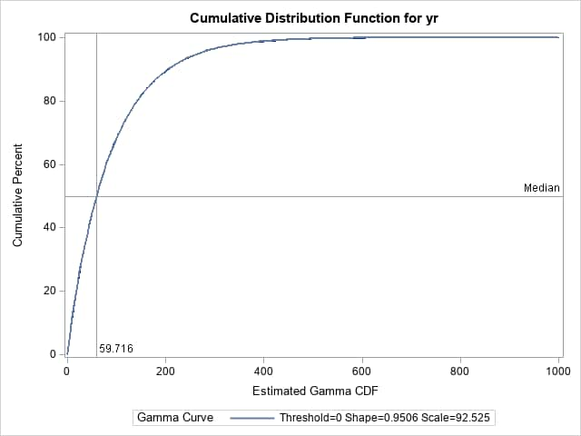
By specifying the GAMMA option and the estimated parameters (scale and λ) in the HISTOGRAM statement below, the UNIVARIATE procedure displays tables describing the specified gamma distribution. The NOPLOT option suppresses the plot of the histogram. The median computed from the random values (59.232) is shown as the 50th percentile in the Observed column of the Quantiles table. The median, as estimated from the gamma distribution with the specified parameters (59.716), appears in the Estimated column. Notice that the median and other quantiles computed from the estimated gamma parameters closely agrees with the median computed from the random values generated from those parameters as you would expect. The CDFPLOT statement plots the cumulative distribution function (CDF) of the random values (the empirical CDF) and overlays the CDF of the specified theoretical gamma distribution. Notice that the curves are essentially identical with no visible gaps between them. Reference lines indicate the median of the estimated distribution.
      proc univariate data=gamsamp noprint;
         var yr;
         histogram yr / noplot gamma(alpha=&scale sigma=&lambda);
         cdfplot yr / gamma(alpha=&scale sigma=&lambda)
                      href=59.716 hreflabel='59.716' hreflabpos=3
                      vref=50     vreflabel='Median';
         label yr="Estimated Gamma CDF";
         run;
 |
Operating System and Release Information
| Product Family | Product | System | SAS Release | |
| Reported | Fixed* | |||
| SAS System | SAS/STAT | z/OS | ||
| OpenVMS VAX | ||||
| Microsoft® Windows® for 64-Bit Itanium-based Systems | ||||
| Microsoft Windows Server 2003 Datacenter 64-bit Edition | ||||
| Microsoft Windows Server 2003 Enterprise 64-bit Edition | ||||
| Microsoft Windows XP 64-bit Edition | ||||
| Microsoft® Windows® for x64 | ||||
| OS/2 | ||||
| Microsoft Windows 95/98 | ||||
| Microsoft Windows 2000 Advanced Server | ||||
| Microsoft Windows 2000 Datacenter Server | ||||
| Microsoft Windows 2000 Server | ||||
| Microsoft Windows 2000 Professional | ||||
| Microsoft Windows NT Workstation | ||||
| Microsoft Windows Server 2003 Datacenter Edition | ||||
| Microsoft Windows Server 2003 Enterprise Edition | ||||
| Microsoft Windows Server 2003 Standard Edition | ||||
| Microsoft Windows XP Professional | ||||
| Windows Millennium Edition (Me) | ||||
| Windows Vista | ||||
| 64-bit Enabled AIX | ||||
| 64-bit Enabled HP-UX | ||||
| 64-bit Enabled Solaris | ||||
| ABI+ for Intel Architecture | ||||
| AIX | ||||
| HP-UX | ||||
| HP-UX IPF | ||||
| IRIX | ||||
| Linux | ||||
| Linux for x64 | ||||
| Linux on Itanium | ||||
| OpenVMS Alpha | ||||
| OpenVMS on HP Integrity | ||||
| Solaris | ||||
| Solaris for x64 | ||||
| Tru64 UNIX | ||||
| Type: | Usage Note |
| Priority: | |
| Topic: | SAS Reference ==> Procedures ==> GENMOD SAS Reference ==> Functions ==> Random Number ==> RAND SAS Reference ==> Functions ==> Probability ==> CDF SAS Reference ==> Procedures ==> UNIVARIATE SAS Reference ==> Functions ==> Probability ==> PDF |
| Date Modified: | 2021-09-07 09:42:29 |
| Date Created: | 2008-08-26 15:38:56 |