Usage Note 22565: Testing for differences in a two-way table with a significant chi-square
 |  |  |
When analysis of a two-way table with multiple rows and/or columns yields a significant chi-square statistic indicating that differences exist among the rows and/or columns, it is usually of interest to perform multiple comparison tests to discover where the differences lie. While there are no formal multiple comparison methods directly available in PROC FREQ, there are a number of approaches that can be used including the following, each of which is discussed below.
Non-model-based methods
- Correspondence analysis is often used as a way to visualize the nonindependence in a table. It can show which rows or columns differ from the others. However, no statistical tests are performed. See the examples in the CORRESP documentation.
- Conducting Pearson chi-square tests on subtables. Use the WHERE statement to select subsets of rows, columns, or both. You can define formats to merge rows or columns if needed. Note, however, that tests on arbitrary subtables will not be independent, and therefore will not partition the chi-square from the original table. It is possible to partition the likelihood ratio chi-square statistic by using certain rules of partitioning the table into a set of 2x2 tables. These rules are outlined in Agresti (2002). Also, because multiple subtables result in multiple tests, adjusting for the multiplicity is important. Consider using the MULTTEST procedure to perform multiplicity-adjusted Fisher or Cochran-Armitage tests. See the MULTTEST documentation and these additional references.
Model-based methods
- When none of the variables can be designated as the response variable with the others as predictors of that response, multiple comparisons can be done by fitting a Poisson loglinear model in PROC GENMOD that allows for nonindependence. With this model, you can then construct custom tests of the desired comparisons. Again, PROC MULTTEST can be used to adjust the p-values from the multiple tests.
- When there is a clearly identifiable response variable, you can fit a logistic model in PROC LOGISTIC and again construct custom comparison tests.
Note that the methods illustrated below are appropriate for comparing proportions from independent proportions, such as from multiple, independent groups of subjects. See this note for comparing dependent proportions, such as the proportions of a multinomial variable observed in a single sample of subjects.
The above methods are illustrated using the table resulting from following data.
      data melanoma;
         input type:$13. site:$11. count;
         cards;
      Hutchinson's  Head         22
      Hutchinson's  Trunk         2
      Hutchinson's  Extremities  10
      Superficial   Head         16
      Superficial   Trunk        54
      Superficial   Extremities 115
      Nodular       Head         19
      Nodular       Trunk        33
      Nodular       Extremities  73
      Indeterminate Head         11
      Indeterminate Trunk        17
      Indeterminate Extremities  28
      ;
Note the significant chi-square test (p<0.0001) that is produced by the CHISQ option in PROC FREQ, indicating lack of independence between TYPE and SITE. The CELLCHI2 option displays the contributions of the cells to the overall chi-square statistic. Note that the Hutchinson's row accounts for the vast majority of the chi-square statistic, indicating that this row differs from the others. Similarly, the Head column accounts for much more of the chi-square statistic than the other two columns, indicating it differs from the others.
      proc freq data=melanoma;
         weight count;
         tables type*site / chisq cellchi2 nopercent;
         run;
Statistics for Table of type by site
|
|||||||||||||||||||||||||||||||||||||||||||||||||||||||||||||||||||||
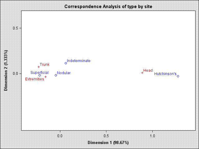
Correspondence analysis
These difference patterns can also be seen by comparing the patterns of row percentages across the rows and comparing the patterns of column percentages across the columns. A correspondence analysis plot makes the differences visually obvious. Note that Hutchinson's and Head are well separated from the other rows and columns, further confirming that this is the nature of the nonindependence within the table.
      ods graphics on;
      proc corresp data=melanoma;
        weight count;
        tables type, site;
        run;
 |
Testing subtables
Pairwise comparisons among the types can be done by running PROC FREQ on each pair of types. Include a WHERE statement in each PROC FREQ step to select the desired pair. This appears to confirm that Hutchinson's differs from the other types. Pairwise comparisons among the columns could be done in a similar fashion.
      ods output chisq(persist)=chisq(where=(statistic="Chi-Square")
                                      rename=(Prob=Raw_P));
      proc freq data=melanoma;
         where type in ("Hutchinson's", "Superficial");
         weight count;
         tables type*site / chisq cellchi2 nopercent;
         run;
      proc freq data=melanoma;
         where type in ("Hutchinson's", "Indeterminate");
         weight count;
         tables type*site / chisq cellchi2 nopercent;
         run;
      proc freq data=melanoma;
         where type in ("Hutchinson's", "Nodular");
         weight count;
         tables type*site / chisq cellchi2 nopercent;
         run;
      proc freq data=melanoma;
         where type in ("Indeterminate", "Nodular");
         weight count;
         tables type*site / chisq cellchi2 nopercent;
         run;
      proc freq data=melanoma;
         where type in ("Indeterminate", "Superficial");
         weight count;
         tables type*site / chisq cellchi2 nopercent;
         run;
      proc freq data=melanoma;
         where type in ("Nodular", "Superficial");
         weight count;
         tables type*site / chisq cellchi2 nopercent;
         run;
      ods output clear;

      proc print noobs;
         var value raw_p;
         run;
|
Adjustment of p-values for the problem of multiple testing can be done in PROC MULTTEST. The ODS OUTPUT statements at the beginning and end of the preceding set of pairwise PROC FREQ steps create a data set called CHISQ that contains the Pearson chi-square results from all of the subtables. The PDATA= option in PROC MULTTEST enables you to read a data set that contains a set of p-values to be adjusted. Since MULTTEST requires that the p-values be in a variable named RAW_P, the RENAME= option is used in the first ODS OUTPUT statement above. Even using the fairly conservative Bonferroni adjustment, the first three tests that compare Hutchinson's with the other types are still significant. The other comparisons show no significant differences.
      proc multtest inpvalues=chisq bon;
         run;
|
||||||||||||||||||||||||
A test of Hutchinson's against the other three types merged together can be done by creating and using a format that groups the three types.
      proc format;
         value $typefmt H-I="Hutchinson's" I-T="Others";
         run;
      proc freq data=melanoma;
         weight count;
         tables type*site / chisq cellchi2 nopercent;
         format type $typefmt.;
         run;
Statistics for Table of type by site
|
|||||||||||||||||||||||||||||||||||||||||||||||||||||||||||
Comparisons in a loglinear model
The same tests of independence as provided by the CHISQ option in PROC FREQ can be obtained by fitting a Poisson loglinear model in PROC GENMOD. The following statements fit the independence model, which includes only the main effects. Nonindependence means that there is some interaction between the row and column variables. The Pearson chi-square statistic that is reported by PROC GENMOD is a test of the interaction and is identical to the chi-square from PROC FREQ run on the full table. Similarly, the Deviance matches the likelihood ratio chi-square from PROC FREQ.
      proc genmod data=melanoma;
         class type site;
         model count=type site / dist=poisson;
         run;
|
||||||||||||||||||||||||||||
Adding the TYPE*SITE interaction in the model enables you to test the nature of the nonindependence by using LSMEANS and LSMESTIMATE statements.Note In the following statements, the TYPE3 and WALD options provide tests of the main effects and interaction. Notice that the test of the interaction is similar to the Deviance in the previous independence model and the likelihood ratio chi-square obtained from PROC FREQ run on the full table.
You can add LSMESTIMATE statements to test the hypothesis that the Hutchinson's row differs from the other rows. For the pattern in Hutchinson's row to be the same as in another row, the differences between Extremities and Head and between Extremities and Trunk should be the same as in the other row. The first three LSMESTIMATE statements that follow jointly test these differences between Hutchinson's and each of the other rows. A set of coefficients in the LSMESTIMATE statement is applied to the LSMEANS in the order shown in the results of the LSMEANS statement. For example, the first set of coefficients in the first LSMESTIMATE statement (1 -1 0 -1 1 0) compares the Extremeties-Head difference in the Hutchinson's row to the same difference in the Indeterminant row. The comparison is done by subtraction which is why the signs reverse in the second set of three values. This same comparison is then done for the Extremities-Trunk difference in the next set of coefficients. Together they compare the patterns in the Hutchinson's and Indeterminant rows. The JOINT(ONLY) option provides a single, combined test. The next two LSMESTIMATE statements are constructed in the same manner.
The final LSMESTIMATE statement is a joint test of the three preceding pairwise comparisons and demonstrates that the pairwise comparisons decompose the interaction. Notice that the test of this final LSMESTIMATE statement matches the TYPE3 test of the full interaction.
The tests from the first three LSMESTIMATE statements give similar chi-squares to those obtained from the previous pairwise runs of PROC FREQ (results not shown) and confirm the difference of the Hutchinson's row from each of the others. LSMESTIMATE statements could similarly be constructed to compare the columns.
      proc genmod data=melanoma;
         class type site;
         model count=type site type*site / dist=poisson type3 wald;
         lsmeans type*site;
         lsmestimate type*site 'Hut vs Ind' 1 -1 0  -1 1 0,
                               'Hut vs Ind' 1 0 -1  -1 0 1 / joint(only);
         lsmestimate type*site "Hut vs Nod" 1 -1 0  0 0 0  -1 1 0,
                               "Hut vs Nod" 1 0 -1  0 0 0  -1 0 1 / joint(only);
         lsmestimate type*site "Hut vs Sup" 1 -1 0  0 0 0  0 0 0  -1 1 0,
                               "Hut vs Sup" 1 0 -1  0 0 0  0 0 0  -1 0 1 / joint(only);
         lsmestimate type*site "Hut vs All" 1 -1 0  -1 1 0,
                               "Hut vs All" 1 0 -1  -1 0 1,
                               "Hut vs All" 1 -1 0  0 0 0  -1 1 0,
                               "Hut vs All" 1 0 -1  0 0 0  -1 0 1,
                               "Hut vs All" 1 -1 0  0 0 0  0 0 0  -1 1 0,
                               "Hut vs All" 1 0 -1  0 0 0  0 0 0  -1 0 1 / joint(only);
         run;
|
||||||||||||||||||||||||||||||||||||||||||||||||||||||||||||||||||||||||||||||||||||||||||||||||||||||||||||||||||||||||||||||||||||||||||||||||||||||||||||||||||||
Comparisons in a logistic model
When one of the variables is considered the response and the other a predictor of that response, then a logistic model can be fit. When the response has several levels which do not have a natural ordering, generalized logits are modeled by specifying the LINK=GLOGIT option in PROC LOGISTIC. In this example, suppose that SITE is treated as the response variable and TYPE as the predictor. The LSMEANS and LSMESTIMATE statements can again be used to make comparisons among the TYPEs. Use of these statements requires the PARAM=GLM option in the CLASS statement.
The following statements fit the generalized logit model and produce the same pairwise comparisons as above of TYPE=Hutchinson's with the other TYPEs. Note that with this model, the specification of the contrast coefficients in the comparisons is considerably simpler because only the TYPE variable is specified in the LSMEANS and LSMESTIMATE statements. The results match those from the loglinear model in the previous section.
      proc logistic data=melanoma;
         freq Count;
         class type / param=glm;
         model site(order=data)=type / link=glogit;
         lsmeans type / diff ;
         lsmestimate type 'Hut v Ind overall' 1 -1 0 0 / category=joint joint(only);
         lsmestimate type 'Hut v Nod overall' 1 0 -1 0 / category=joint joint(only);
         lsmestimate type 'Hut v Sup overall' 1 0 0 -1 / category=joint joint(only);
         lsmestimate type 'Hut v Ind overall' 1 -1 0 0,
                          'Hut v Nod overall' 1 0 -1 0,
                          'Hut v Sup overall' 1 0 0 -1 / category=joint joint(only);
         run;
________
Note: CONTRAST statements can also be used and provide likelihood ratio tests instead of Wald tests. However, the process for correctly determining contrast coefficients is generally more difficult. To determine the coefficients needed in the CONTRAST statement, it is necessary to write out the form of the model that you are fitting in PROC GENMOD, and then write out the hypothesis to be tested in terms of the model parameters and simplify. This process applies to CONTRAST and ESTIMATE statements in all modeling procedures and is discussed and illustrated in detail in Examples of Writing CONTRAST and ESTIMATE Statements. The likelihood ratio tests produced by the contrasts match the likelihood ratio chi-squares that are obtained from the previous pairwise runs of PROC FREQ (results not shown) and confirm the difference of the Hutchinson's row from each of the others. Contrasts could similarly be constructed to compare the columns.
      proc genmod data=melanoma;
         class type site;
         model count=type site type*site / dist=poisson type3;
         contrast "Hut vs Ind" type*site 1 -1 0  -1 1 0,
                               type*site 1 0 -1  -1 0 1;
         contrast "Hut vs Nod" type*site 1 -1 0  0 0 0  -1 1 0,
                               type*site 1 0 -1  0 0 0  -1 0 1;
         contrast "Hut vs Sup" type*site 1 -1 0  0 0 0  0 0 0  -1 1 0,
                               type*site 1 0 -1  0 0 0  0 0 0  -1 0 1;
         contrast "Hut vs All" type*site 1 -1 0  -1 1 0,
                               type*site 1 0 -1  -1 0 1,
                               type*site 1 -1 0  0 0 0  -1 1 0,
                               type*site 1 0 -1  0 0 0  -1 0 1,
                               type*site 1 -1 0  0 0 0  0 0 0  -1 1 0,
                               type*site 1 0 -1  0 0 0  0 0 0  -1 0 1;
         run;
Operating System and Release Information
| Product Family | Product | System | SAS Release | |
| Reported | Fixed* | |||
| SAS System | SAS/STAT | All | n/a | |
| Type: | Usage Note |
| Priority: | low |
| Topic: | SAS Reference ==> Procedures ==> MULTTEST SAS Reference ==> Procedures ==> CORRESP Analytics ==> Psychometrics SAS Reference ==> Procedures ==> FREQ SAS Reference ==> Procedures ==> GENMOD Analytics ==> Categorical Data Analysis Analytics ==> Descriptive Statistics SAS Reference ==> Procedures ==> LOGISTIC |
| Date Modified: | 2020-06-24 10:39:48 |
| Date Created: | 2002-12-16 10:56:38 |