| Variable Transformations |
Transformations for Proportion Variables
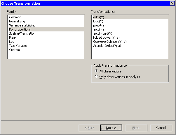
Figure 32.14 shows the transformations that are available
when you select For proportions from the Family list.
These transformations are intended
for variables that represent proportions. That is, the ![]() variable must
take values between 0 and 1. You can also use these transformations
for percentages if you first divide the percentages by 100.
variable must
take values between 0 and 1. You can also use these transformations
for percentages if you first divide the percentages by 100.
Chapter 7 of Atkinson (1985) is devoted to transformations of proportions.
Equations for these transformations are
given in Table 32.4.
|
Figure 32.14: Transformations for Proportions
| Default | Name of | ||
|---|---|---|---|
| Transformation | Parameter | New Variable | Equation |
| odds(Y) | Odds_Y | ||
| logit(Y) | Logit_Y | ||
| probit(Y) | Probit_Y | ||
| arcsin(Y) | Arcsin_Y | ||
| arcsin(sqrt(Y)) | Angular_Y | ||
| folded power(Y;a) | MLE | FPow_Y | See text. |
| Guerrero-Johnson(Y;a) | MLE | GJ_Y | See text. |
| Aranda-Ordaz(Y;a) | MLE | AO_Y | See text. |
The probit function is the quantile function of the standard normal distribution.
The last three transformations in the list are similar to the Box-Cox
transformation described in the section "Normalizing Transformations". The
parameter for each transformation is in the unit interval:
![]() . Typically, you choose a parameter that maximizes (or
nearly maximizes) a log-likelihood function.
. Typically, you choose a parameter that maximizes (or
nearly maximizes) a log-likelihood function.
The log-likelihood function is defined
as follows. Let ![]() be the
number of nonmissing values, and let
be the
number of nonmissing values, and let ![]() be the
geometric mean function.
Each transformation has a corresponding normalized transformation
be the
geometric mean function.
Each transformation has a corresponding normalized transformation
![]() , to be defined later.
Define
, to be defined later.
Define
The following sections define the normalized transformation for the
folded power, Guerrero-Johnson, and Aranda-Ordaz transformations.
In each section, ![]() .
.
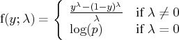
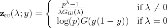
The Folded Power Transformation
The folded power transformation is defined as
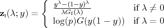
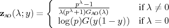
The Guerrero-Johnson Transformation
The Guerrero-Johnson transformation is defined as
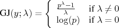
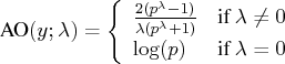
The Aranda-Ordaz Transformation
The Aranda-Ordaz transformation is defined as
Copyright © 2008 by SAS Institute Inc., Cary, NC, USA. All rights reserved.