The Data Table

Variable Properties

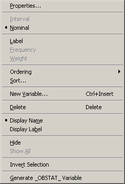
You can change the properties of a variable by using the Variables menu, as shown in Figure 4.2. You can access the Variables menu by clicking on the column heading and selecting Edit $\blacktriangleright\,$ Variables from the main menu. Alternatively, right-clicking on a variable heading (see Figure 4.1) selects that variable and displays the same menu.

You can use the Variables menu to do the following:

change properties of existing variables
set the role of an existing variable
create a new variable
change the set of variables that are displayed in the data table
change the set of selected and unselected variables

One variable property that might be unfamiliar is the role. You can assign three default roles:

Label: The values of the variable are used to label clicked-on markers in plots.
Frequency: The values of the variable are used as the frequency of occurrence for each observation.
Weight: The values of the variable are used as weights for each observation.

If you assign a variable to a Frequency role, then that variable is automatically added to dialog boxes for analyses and graphs that support a frequency variable. The same is true for variables with a Weight role.

There can be at most one variable for each role. A variable can play multiple roles.

Figure 4.2: The Variables Menu

The following list describes each item on the variable menu.

Properties

displays the Variable Properties dialog box, described in the section "Adding Variables". The dialog box enables you to change most properties for the selected variable. However, you cannot change the type (character or numeric) of an existing variable.

Interval/Nominal

changes the measure level of the selected numeric variable. A character variable cannot be interval.

Label

makes the selected variable the label variable for plots.

Frequency

makes the selected variable the frequency variable for analyses and plots that support a frequency variable. Only numeric variables can have a Frequency role.

Weight

makes the selected variable the weight variable for analyses and plots that support a weight variable. Only numeric variables can have a Weight role.

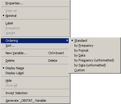
Ordering

specifies how nominal variables are ordered. This affects the way that a variable is sorted and the order of categories in plots. If a variable has missing values, they are always ordered first. See the section "Ordering Categories of a Nominal Variable" for further details. The Ordering submenu is shown in Figure 4.3. You can order a variable in the following ways:

Standard: specifies that categories are arranged in ASCII order by their unformatted values. In ASCII order, numerals precede uppercase letters, which precede lowercase letters.
by Frequency: specifies that categories are arranged according to the descending frequency count of formatted values in each category.
by Format: specifies that categories are arranged in ASCII order by their formatted values.
by Data: specifies that categories are arranged according to the data order of formatted values. The data order is determined by traversing the values of a variable, starting from the first observation. The first (nonmissing) value you encounter is ordered first, the next unique (nonmissing) value of the variable is ordered second, and so on. Sorting the data table does not affect this ordering; it is based on the original order of observations.
by Frequency (unformatted): specifies that categories are arranged according to the descending frequency count of unformatted values in each category.
by Data (unformatted): specifies that categories are arranged according to the data order of unformatted values. Sorting the data table does not affect this ordering; it is based on the original order of observations.
Custom: specifies that this variable was ordered by calling the DataObject.SetVarValueOrder method. See the Stat Studio online Help for details about this method.

Sort

displays the Sort dialog box. The Sort dialog box is described in the section "Sorting Observations".

New Variable

displays the New Variable dialog box (Figure 3.5) to create a new variable as described in the section "Adding Variables".

Delete

deletes the selected variables.

Display Name/Display Label

toggles whether the column heading displays the name of variables or displays their labels.

Hide

hides the selected variables. The variables can be displayed at a later time by selecting Show All. Hidden variables cannot be selected.

Show All

displays all variables, including variables that were hidden.

Invert Selection

changes the set of selected variables. Unselected variables become selected, while selected variables become unselected.

Generate _OBSTAT_ Variable

creates a new character variable called _OBSTAT_ that encodes the current state of each observation. The values of the _OBSTAT_ variable are described in the following paragraphs.

Figure 4.3: The Ordering Menu

The _OBSTAT_ variable is a character variable of length 20. It was introduced in SAS/INSIGHT software as a way to capture the state of observations, including the color and shape of markers and whether an observation is selected. The first few characters encode the state of binary options such as whether an observation is selected. A character is '1' if the corresponding property is true and '0' if the related property is false. The properties are described in the following list:

Character 1: stores whether the observation is selected.

Character 2

stores whether the observation is included in plots.

Character 3

stores whether the observation is included in analyses.

Character 4

stores whether the observation has a label.

Character 5

stores the marker shape for an observation. This is a value between 1 and 8 that corresponds to a shape, as given in the following table:

Value	Shape
1	$\box$
2
3	$\circ$
4	$\diamond$
5
6	$\bigtriangleup$
7	$\bigtriangledown$
8	$\star$

Characters 6 - 20

store the RGB value of the fill color for an observation marker. The RGB color model represents colors as combinations of the colors red, green, and blue.

Each component is a five-digit decimal number between 0 and 65535. Characters 6 - 10 store the red component. Characters 11 - 15 store the green component. Characters 16 - 20 store the blue component.

If you read a data set for which there is no associated DMM file, and if that data set contains a variable named _OBSTAT_, then the state of each observation is determined by the corresponding value of the _OBSTAT_ variable.

If an _OBSTAT_ variable already exists when you select Generate _OBSTAT_ Variable from the variable menu, then the values of the variable are updated with the current state of the observations.

The _OBSTAT_ variable is often used to analyze observations with certain properties by using a SAS procedure. To use the _OBSTAT_ variable outside Stat Studio, you can do the following:

Create an _OBSTAT_ variable by selecting Generate _OBSTAT_ Variable from the variable menu.
Save the augmented data set to a libref such as SASUSER.

Use the following DATA step to extract each observation property into its own variable:

  
    /* Create numerical variables from an _OBSTAT_ variable. */ 
    data MyData; 
    set sasuser.MyData; 
    IsSelected   = inputn(substr(_obstat_,  1, 1), 1.); 
    IsInPlots    = inputn(substr(_obstat_,  2, 1), 1.); 
    IsInAnalysis = inputn(substr(_obstat_,  3, 1), 1.); 
    IsLabeled    = inputn(substr(_obstat_,  4, 1), 1.); 
    MarkerShape  = inputn(substr(_obstat_,  5, 1), 1.); 
    MarkerRed    = inputn(substr(_obstat_,  6, 5), 5.); 
    MarkerGreen  = inputn(substr(_obstat_, 11, 5), 5.); 
    MarkerBlue   = inputn(substr(_obstat_, 16, 5), 5.); 
    run;

Use a WHERE clause to analyze only observations with a given set of properties.

Top of Page