The SURVEYREG Procedure

Suppose that the previous student sample is actually selected by using a stratified sample design. The strata are the grades in the junior high school: 7, 8, and 9. Within the strata, simple random samples are selected. Table 114.1 provides the number of students in each grade.

In order to analyze this sample by using PROC SURVEYREG, you need to input the stratification information by creating a SAS data set that contains the information in Table 114.1. The following SAS statements create such a data set, named StudentTotals:

data StudentTotals;
   input Grade _TOTAL_; 
   datalines;
7 1824
8 1025
9 1151
;

The variable Grade is the stratification variable, and the variable _TOTAL_ contains the total numbers of students in each stratum in the survey population. PROC SURVEYREG requires you to use the keyword _TOTAL_ as the name of the variable that contains the population totals.

When the sample design is stratified and the stratum sampling rates are unequal, you should use sampling weights to reflect this information in the analysis. For this example, the appropriate sampling weights are the reciprocals of the probabilities of selection. You can use the following DATA step to create the sampling weights:

data IceCream; 
   set IceCream; 
   if Grade=7 then Prob=20/1824;
   if Grade=8 then Prob=9/1025;
   if Grade=9 then Prob=11/1151;
   Weight=1/Prob;
run;

If you use PROC SURVEYSELECT to select your sample, PROC SURVEYSELECT creates these sampling weights for you.

The following statements demonstrate how you can fit a linear model while incorporating the sample design information (stratification and unequal weighting):

ods graphics on;
title1 'Ice Cream Spending Analysis';
title2 'Stratified Sample Design';
proc surveyreg data=IceCream total=StudentTotals;
   strata Grade /list;
   model Spending = Income;
   weight Weight;
run;

Comparing these statements to those in the section Simple Random Sampling, you can see how the TOTAL=StudentTotals option replaces the previous TOTAL=4000 option.

The STRATA statement specifies the stratification variable Grade. The LIST option in the STRATA statement requests that the stratification information be displayed. The WEIGHT statement specifies the weight variable.

Figure 114.4 summarizes the data information, the sample design information, and the fit information. Because of the stratification, the denominator degrees of freedom for F tests and t tests are 37, which are different from those in the analysis in Figure 114.1.

Figure 114.5 displays the following information for each stratum: the value of the stratification variable, the number of observations (sample size), the total population size, and the sampling rate (fraction).

Figure 114.6 displays the tests for significance of the model effects. The Income effect is strongly significant at the 5% level.

Figure 114.7 displays the regression coefficient estimates, their standard errors, and the associated t tests for the stratified sample.

You can request other statistics and tests by using PROC SURVEYREG. You can also analyze data from a more complex sample design. The remainder of this chapter provides more detailed information.

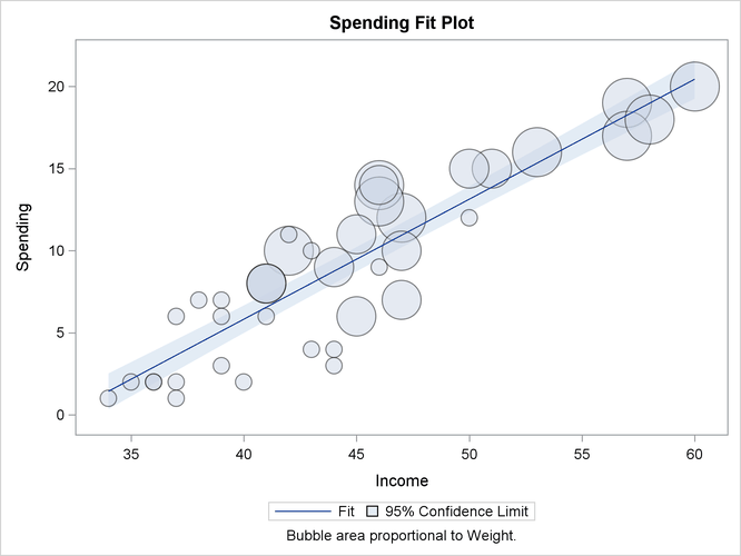
When ODS Graphics is enabled and the model contains a single continuous regressor, PROC SURVEYREG provides a fit plot that displays the regression line and the confidence limits of the mean predictions. Figure 114.8 displays the fit plot for the regression model of Spending as a function of Income. The regression line and confidence limits of mean prediction are overlaid by a bubble plot of the data, in which the bubble area is proportional to the sampling weight of an observation.

Figure 114.8: Regression Fitting