The SURVEYREG Procedure
- Overview
-
Getting Started

-
SyntaxPROC SURVEYREG StatementBY StatementCLASS StatementCLUSTER StatementCONTRAST StatementDOMAIN StatementEFFECT StatementESTIMATE StatementLSMEANS StatementLSMESTIMATE StatementMODEL StatementOUTPUT StatementREPWEIGHTS StatementSLICE StatementSTORE StatementSTRATA StatementTEST StatementWEIGHT Statement
-
Details
-
Examples
- References
Example 114.4 Stratified Sampling
This example illustrates the use of the SURVEYREG procedure to perform a regression in a stratified sample design. Consider
a population of 235 farms producing corn in Nebraska and Iowa. You are interested in the relationship between corn yield (CornYield) and total farm size (FarmArea).
Each state is divided into several regions, and each region is used as a stratum. Within each stratum, a simple random sample with replacement is drawn. A total of 19 farms is selected by using a stratified simple random sample. The sample size and population size within each stratum are displayed in Table 114.12.
Table 114.12: Number of Farms in Each Stratum
|
Number of Farms |
||||
|---|---|---|---|---|
|
Stratum |
State |
Region |
Population |
Sample |
|
1 |
Iowa |
1 |
100 |
3 |
|
2 |
2 |
50 |
5 |
|
|
3 |
3 |
15 |
3 |
|
|
4 |
Nebraska |
1 |
30 |
6 |
|
5 |
2 |
40 |
2 |
|
|
Total |
235 |
19 |
||
The following three models are considered:
-
Model I — Common intercept and slope:
![\[ \mbox{Corn Yield}=\alpha +\beta *\mbox{Farm Area} \]](images/statug_surveyreg0120.png)
-
Model II — Common intercept, different slope:
![\[ \mbox{Corn Yield} =\left\{ {\begin{array}{ll} \alpha +\beta _{\mbox{Iowa}}*\mbox{Farm Area} & \mbox{if the farm is in Iowa} \\ \alpha +\beta _{\mbox{Nebraska}}*\mbox{Farm Area} & \mbox{if the farm is in Nebraska} \end{array} } \right. \]](images/statug_surveyreg0121.png)
-
Model III — Different intercept and different slope:
![\[ \mbox{Corn Yield}=\left\{ {\begin{array}{ll} \alpha _{\mbox{Iowa}}+\beta _{\mbox{Iowa}}*\mbox{Farm Area} & \mbox{if the farm is in Iowa} \\ \alpha _{\mbox{Nebraska}}+\beta _{\mbox{Nebraska}}* \mbox{Farm Area} & \mbox{if the farm is in Nebraska} \end{array}} \right. \]](images/statug_surveyreg0122.png)
Data from the stratified sample are saved in the SAS data set Farms. The variable Weight contains the sampling weights, which are reciprocals of the selection probabilities.
data Farms;
   input State $ Region FarmArea CornYield Weight;
   datalines;
Iowa     1 100  54 33.333
Iowa     1  83  25 33.333
Iowa     1  25  10 33.333
Iowa     2 120  83 10.000
Iowa     2  50  35 10.000
Iowa     2 110  65 10.000
Iowa     2  60  35 10.000
Iowa     2  45  20 10.000
Iowa     3  23   5  5.000
Iowa     3  10   8  5.000
Iowa     3 350 125  5.000
Nebraska 1 130  20  5.000
Nebraska 1 245  25  5.000
Nebraska 1 150  33  5.000
Nebraska 1 263  50  5.000
Nebraska 1 320  47  5.000
Nebraska 1 204  25  5.000
Nebraska 2  80  11 20.000
Nebraska 2  48   8 20.000
;
The SAS data set StratumTotals contains the stratum population sizes.
data StratumTotals;
   input State $ Region _TOTAL_;
   datalines;
Iowa     1 100
Iowa     2  50
Iowa     3  15
Nebraska 1  30
Nebraska 2  40
;
Using the sample data from the data set Farms and the control information data from the data set StratumTotals, you can fit Model I by using the following statements in PROC SURVEYREG:
ods graphics on;
title1 'Analysis of Farm Area and Corn Yield';
title2 'Model I: Same Intercept and Slope';
proc surveyreg data=Farms total=StratumTotals;
   strata State Region / list;
   model CornYield = FarmArea / covB;
   weight Weight;
run;
Output 114.4.1 displays the data summary and stratification information fitting Model I. The sampling rates are automatically computed by the procedure based on the sample sizes and the population totals in strata.
Output 114.4.1: Data Summary and Stratum Information Fitting Model I
Output 114.4.2 displays tests of model effects and the estimated regression coefficients.
Output 114.4.2: Estimated Regression Coefficients and the Estimated Covariance Matrix
Output 114.4.3: Regression Fitting
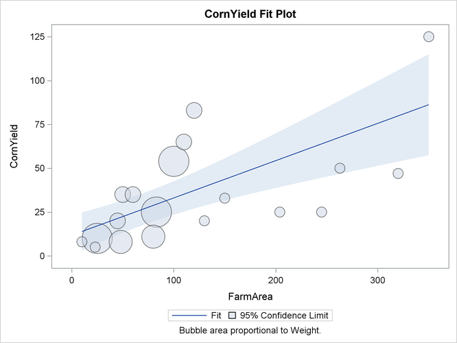
Output 114.4.3 displays the fit of the regression.
Alternatively, you can assume that the linear relationship between corn yield (CornYield) and farm area (FarmArea) is different among the states (Model II). In order to analyze the data by using this model, you create auxiliary variables
FarmAreaNE and FarmAreaIA to represent farm area in different states:
![\[ \Variable{FarmAreaNE}=\left\{ {\begin{array}{ll} 0 & \mbox{if the farm is in Iowa} \\ \Variable{FarmArea} & \mbox{if the farm is in Nebraska} \end{array} } \right. \]](images/statug_surveyreg0123.png)
![\[ \Variable{FarmAreaIA}=\left\{ {\begin{array}{ll} \Variable{FarmArea} & \mbox{if the farm is in Iowa} \\ 0 & \mbox{if the farm is in Nebraska} \end{array} } \right. \]](images/statug_surveyreg0124.png)
The following statements create these variables in a new data set called FarmsByState and use PROC SURVEYREG to fit Model II:
data FarmsByState;
   set Farms;
   if State='Iowa' then do;
      FarmAreaIA=FarmArea;
      FarmAreaNE=0;
   end;

   else do;
      FarmAreaIA=0;
      FarmAreaNE=FarmArea;
   end;
run;
The following statements perform the regression by using the new data set FarmsByState. The analysis uses the auxiliary variables FarmAreaIA and FarmAreaNE as the regressors:
title1 'Analysis of Farm Area and Corn Yield';
title2 'Model II: Same Intercept, Different Slopes';
proc surveyreg data=FarmsByState total=StratumTotals;
   strata State Region;
   model CornYield = FarmAreaIA FarmAreaNE / covB;
   weight Weight;
run;
Output 114.4.4 displays the fit statistics and parameter estimates. The estimated slope parameters for each state are quite different from the estimated slope in Model I. The results from the regression show that Model II fits these data better than Model I.
Output 114.4.4: Regression Results from Fitting Model II
For Model III, different intercepts are used for the linear relationship in two states. The following statements illustrate the use of the NOINT option in the MODEL statement associated with the CLASS statement to fit Model III:
title1 'Analysis of Farm Area and Corn Yield';
title2 'Model III: Different Intercepts and Slopes';
proc surveyreg data=FarmsByState total=StratumTotals;
   strata State Region;
   class State;
   model CornYield = State FarmAreaIA FarmAreaNE / noint covB solution;
   weight Weight;
run;
The model statement includes the classification effect State as a regressor. Therefore, the parameter estimates for effect State present the intercepts in two states.
Output 114.4.5 displays the regression results for fitting Model III, including parameter estimates, and covariance matrix of the regression coefficients. The estimated covariance matrix shows a lack of correlation between the regression coefficients from different states. This suggests that Model III might be the best choice for building a model for farm area and corn yield in these two states.
However, some statistics remain the same under different regression models—for example, Weighted Mean of CornYield. These estimators do not rely on the particular model you use.
Output 114.4.5: Regression Results for Fitting Model III
| Estimated Regression Coefficients | ||||
|---|---|---|---|---|
| Parameter | Estimate | Standard Error |
t Value | Pr > |t| |
| State Iowa | 5.27797099 | 5.27170400 | 1.00 | 0.3337 |
| State Nebraska | 0.65275201 | 1.70031616 | 0.38 | 0.7068 |
| FarmAreaIA | 0.40680971 | 0.06458426 | 6.30 | <.0001 |
| FarmAreaNE | 0.14630563 | 0.01997085 | 7.33 | <.0001 |
| Note: | The degrees of freedom for the t tests is 14. |