The LIFETEST Procedure

Kernel-Smoothed Hazard Estimate
Kernel-smoothed estimators of the hazard function  are based on the Nelson-Aalen estimator
  and its variance
  . Consider the jumps of and at the event times
 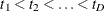 as follows:
where  =0.
=0.
The kernel-smoothed estimator of is a weighted average of  over event times that are within a bandwidth distance b of t. The weights are controlled by the choice of kernel function,
  , defined on the interval [–1,1]. The choices are as follows:
-
uniform kernel:
![\[ K_ U(x) = \frac{1}{2}, ~ ~ -1\leq x \leq 1\\ \]](images/statug_lifetest0173.png)
-
Epanechnikov kernel:
![\[ K_ E(x) = \frac{3}{4}(1-x^2), ~ ~ -1\leq x \leq 1 \]](images/statug_lifetest0174.png)
-
biweight kernel:
![\[ K_{\mi{BW}}(x) = \frac{15}{16}(1-x^2)^2, ~ ~ -1\leq x \leq 1 \]](images/statug_lifetest0175.png)
The kernel-smoothed hazard rate estimator is defined for all time points on  . For time points t for which
  , the kernel-smoothed estimated of based on the kernel is given by
![\[ \hat{h}(t) = \frac{1}{b} \sum _{i=1}^ D K \biggl (\frac{t-t_ i}{b} \biggr ) \Delta \tilde{H}(t_ i) \]](images/statug_lifetest0178.png)
The variance of  is estimated by
![\[ \hat{\sigma ^2}(\hat{h}(t)) = \frac{1}{b^2} \sum _{i=1}^ D K\biggl (\frac{t-t_ i}{b} \biggr )^2 \Delta \hat{V}(\tilde{H}(t_ i)) \]](images/statug_lifetest0180.png)
For t < b, the symmetric kernels are replaced by the corresponding asymmetric kernels of Gasser and Müller (1979). Let  . The modified kernels are as follows:
-
uniform kernel:
![\[ K_{U,q}(x) = \frac{4(1+q^3)}{(1+q)^4} + \frac{6(1-q)}{(1+q)^3}x, ~ ~ ~ -1 \leq x \leq q \]](images/statug_lifetest0182.png)
-
Epanechnikov kernel:
![\[ K_{E,q}(x)= K_ E(x) \frac{64(2-4q+6q^2-3q^3) + 240(1-q)^2 x }{ (1+q)^4(19-18q+3q^2)}, ~ ~ -1 \leq x \leq q \]](images/statug_lifetest0183.png)
-
biweight kernel:
![\[ K_{\mi{BW},q}(x) = K_{\mi{BW}}(x) \frac{64(8-24q+48q^2-45q^3+15q^4) + 1120(1-q)^3 x}{(1+q)^5(81-168q+126q^2-40q^3+5q^4)}, ~ ~ -1\leq x \leq q \]](images/statug_lifetest0184.png)
For  , let
, let  . The asymmetric kernels for
  are used with x replaced by –x.
Using the log transform on the smoothed hazard rate, the 100(1– )% pointwise confidence interval for the smoothed hazard rate is given by
![\[ \hat{h}(t) = \hat{h}(t)\exp \biggl [\pm \frac{z_{1-\alpha /2} \hat{\sigma }(\hat{h}(t))}{\hat{h}(t)} \biggr ] \]](images/statug_lifetest0188.png)
where  is the (100(1–
 ))th percentile of the standard normal distribution.
Optimal Bandwidth
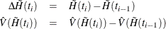
The following mean integrated squared error (MISE) over the range  and
and  is used as a measure of the global performance of the kernel function estimator:
The last term is independent of the choice of the kernel and bandwidth and can be ignored when you are looking for the best
value of b. The first integral can be approximated by using the trapezoid rule by evaluating at a grid of points  . You can specify
  , and M by using the options GRIDL=, GRIDU=, and NMINGRID=, respectively, of the HAZARD plot. The second integral can be estimated
by the Ramlau-Hansen (1983a, 1983b) cross-validation estimate:
, and M by using the options GRIDL=, GRIDU=, and NMINGRID=, respectively, of the HAZARD plot. The second integral can be estimated
by the Ramlau-Hansen (1983a, 1983b) cross-validation estimate:
![\[ \frac{1}{b} \sum _{i \neq j} K\biggl ( \frac{t_ i-t_ j}{b} \biggr ) \Delta \hat{H}(t_ i) \Delta \hat{H}(t_ j) \]](images/statug_lifetest0195.png)
Therefore, for a fixed kernel, the optimal bandwidth is the quantity b that minimizes
![\[ g(b) = \sum _{i=1}^{M-1} \biggl [\frac{u_{i+1} - u_ k}{2} \biggl (\hat{h}^2(u_ i) + \hat{h}^2(u_{i+1}) \biggr )\biggr ] - \frac{2}{b} \sum _{i \neq j} K\biggl ( \frac{t_ i-t_ j}{b} \biggr ) \Delta \hat{H}(t_ i) \Delta \hat{H}(t_ j) \]](images/statug_lifetest0196.png)
The minimization is carried out by the golden section search algorithm.